Concurrent composition in the bounded quantum storage model

(1)

Concurrent composition in the

bounded quantum storage model

∗

Dominique Unruh

University of Tartu, Estonia

May 15, 2011

Abstract

We define the BQS-UC model, a variant of the UC model, that deals with protocols in the bounded quantum storage model. We present a statistically secure commitment protocol in the BQS-UC model that composes concurrently with other protocols and an (a-priori) polynomially-bounded number of instances of itself. Our protocol has an efficient simulator which is important if one wishes to compose our protocol with protocols that are only computationally secure. Combining our result with prior results, we get a statistically BQS-UC secure protocol for general two-party computation without the need for any setup assumption. The round complexity of that protocol is linear in the circuit depth.

1 Introduction

Since the inception of quantum key distribution by Bennett and Brassard [BB84], it has been known that quantum communication permits to achieve protocol tasks that are impossible given only a classical channel. For example, a quantum key distribution scheme [BB84] permits to agree on a secret key that is statistically secret, using only an authenticated but not secret channel. (By statistical security we mean security against computationally unbounded adversaries, also known as information-theoretical security.) In contrast, when using only classical communication, it is easy to see that such a secret key can always be extracted by a computationally sufficiently powerful adversary. In light of this result, one might hope that quantum cryptography allows to circumvent other classical impossibility results, possibly even allowing for statistically secure multi-party computation protocols. Yet, Mayers [May97] showed that also in the quantum setting, even statistically secure commitment schemes are impossible, let alone general multi-party computation. This is unfortunate, because from commitments one can build OT (Bennett, Brassard, Cr´epeau, and Skubiszewska [BBCS91]), and from OT general multi-party computation (Kilian [Kil88]). A way to work around this impossibility was found by Damg˚ard, Fehr, Salvail, and Schaffner [DFSS05]. They showed that if we assume that the quantum memory available to the adversary is bounded (we speak of bounded quantum storage (BQS)), we can construct statistically secure commitment and OT schemes. Although such a result is not truly unconditional, it avoids hard-to-justify complexity-theoretic assumptions. Also, it achieves long-term security: even if the adversary can surpass the memory bound after the protocol execution, this will not allow him to retroactively break the protocol.

Yet, we still have not reached the goal of statistically secure multi-party computation. Although we have protocols for commitment and OT, we cannot simply plug them into the protocols by Bennett et al. [BBCS91] and by Kilian [Kil88]. The reason is that it is not clear under which circumstances protocols in the BQS model may be composed. For exam-ple, Dziembowski and Maurer [DM04] constructed a protocol that is secure in the classical bounded storage model, but that looses security when composed with a computationally secure protocol. To overcome this remaining difficulty, works by Wehner and Wullschleger [WW08] and by Fehr and Schaffner [FS09] give security definitions in the BQS model that enable secure sequential composition. Both works also present secure OT protocols in their respective settings. Based on these, we can construct secure multi-party computation proto-cols in the BQS model. There are, however, a few limitations. First, since only sequential composition is supported, all instances of the OT protocol used by the multi-party compu-tation need to be executed one after another, leading to a high round-complexity. Second, interactive functionalities such as a commitment are difficult to use: the restriction to se-quential composability requires that we have to commit and immediately open a commitment before being allowed to execute the next commitment. Third, the security proof of their OT protocols uses a computationally unlimited simulator. As discussed in [Unr10], a protocol with an unlimited simulator cannot be composed with a computationally secure protocol. Fourth, since we have no concurrent composability, it is not clear what happens if the proto-cols are executed in an environment where we do not have total control about which protoproto-cols are executed at what time.

(3)

and by Unruh [Unr04, Unr10]. In light of the success of the UC model, it seems natural to combine the ideas of the UC model with those of the BQS model in order to allow for concurrent composition.

1.1 Our contribution.

We define the notion of BQS-UC-security, which is an extension of quantum-UC-security [Unr10]. We have composability in the following sense: If π is a secure realization of a functionality F, and σF securely realizes G by using one instance of F, then σπ, the result of replacing F by π, still securely realizes G. In contrast to quantum-UC-security, however, BQS-UC-security does not allow for concurrent self-composition: ifπis secure, this does not automatically imply that two concurrent instances ofπ are secure.1

In order to get protocols that even self-compose concurrently, we design a commitment scheme πCOM such that n concurrent instances of πCOM securely realize n instances of the

commitment functionality in the presence of a-memory bounded adversaries. Here aand n

are arbitrary (polynomially-bounded), but the protocol depends onaand n.

The challenging part in the construction of πCOM is that BQS-UC-security requires the

following: There must be an efficient simulator (which is allowed to have more quantum memory than the adversary) that can extract the committed value (extractability) or change it after the commit phase (equivocality). Prior constructions of commitment schemes in the BQS model required computationally unbounded simulators. Also, the fact that we directly analyze the concurrent composition of several instances ofπCOM requires care: In the proof,

we have hybrid networks in which instances of both πCOM and of the simulator occur. Since

the simulator uses more quantum memory than πCOM tolerates, one needs to ensure that

the simulator cannot be (mis)used by the adversary to break the commitment.

Finally, using the composition theorem andπCOM, for any two-party functionalityG, we

get a statistically secure protocol π realizing G in the BQS model.2 The protocol is secure even when runningnconcurrent instances of the protocol. (Again, this holds for anyn and any memory bound, but the protocol depends on n and the memory-bound.) The round-complexity of the protocol is linear in the circuit depth. It does not use any quantum memory or quantum computation and thus is in the reach of today’s technology.

1.2 Preliminaries

General. A nonnegative function µ is called negligible if for all c > 0 and all sufficiently large k,µ(k)< k−c. µ is called exponentially-small if for somec >0 and sufficiently largek,

µ(k)< c−k_{. A nonnegative function}_f _{is called overwhelming if}_f _≥₁₋_µ_{for some negligible}

µ. Keywords in typewriter font (e.g., environment) are assumed to be fixed but arbitrary distinct non-empty words in{0,1}∗. ε∈ {0,1}∗ denotes the empty word. We write kfor the concatenation of bitstrings. Given a bitstring x, we write xI for x restricted to the indices

in the setI. Given a set M, we writeM∁ for its complement. Ab-block (m, κ, d)-linear code is a code with alphabet{0,1}b _{(that is, each symbol of the code is a}_b_{-bit string), codewords}

1_{The reader may wonder how it can be that}_σ_and_π_{may compose in general while}_π_and_π_{do not. Might}

notσ andπbe the same protocol? The reason lies in the exact conditions of the composition theorem: In order to compose,σ needs to be secure against adversaries with a higher quantum memory bound than π

tolerates. Thusσandπcannot be the same protocol.

2_{We are restricted to two-party functionalities because our construction uses a subprotocol by Wolf and}

(4)

of length m (i.e., mb bits), size 2bκ, and detectingd−1 errors (i.e., any non-zero codeword contains at least d non-zero blocks). The Hamming distance between x and x∗ _{we denote}

ω(x, x∗). (In the case of a block code, this is the number of blocks, not bits, that differ.) We say a family of (m, κ, d)-linear codes, parametrized by a security parameter k, has efficient error-correction if for any x, the codeword x∗ _with _ω₍_{x, x}∗₎ _≤ ₍_d₋₁₎_/_{2 can be found in} deterministic time polynomial in k(if such an x∗ exists).

Quantum systems. We can only give a terse overview over the formalism used in quantum computing. For a thorough introduction, we recommend the textbook by Nielsen and Chuang [NC00, Chap. 1–2]. A (pure) state in a quantum system is described by a vector |ψi in some Hilbert space H. In this work, we only use Hilbert spaces of the form H = C

N _for

some countable set N, usually N = {0,1} for qubits or N = {0,1}∗ _{for bitstrings. We} always assume a designated orthonormal basis {|xi :x ∈N} for each Hilbert space, called the computational basis. The basis states |xi represent classical states (i.e., states without superposition). Given several separate subsystems H1 = C

N1_{, . . . ,}_H

n =C

Nn_{, we describe}

the joint system by the tensor productH1⊗· · ·⊗Hn=C

N1×···×Nn_{. We write}_h_Ψ_|_{for the linear}

transformation mapping|Φi to the scalar producthΨ|Φi. Consequently, |ΨihΨ|denotes the orthogonal projector on |Ψi. We set |0i+ := |0i, |1i+ := |1i, |0i× := √1₂(|0i+|1i), and

|1i_×:= √1

2(|0i − |1i). Forx∈ {0,1}

n_and_θ_{∈ {}₊_,_×}n_{, we define}_|_x_i

θ :=|x1iθ1⊗ · · · ⊗ |xniθn.

Mixed states. If a system is not in a single pure state, but instead is in the pure state

|Ψii ∈ Hwith probabilitypi (i.e., it is in a mixed state), we describe the system by a density

operator ρ = P

ipi|ΨiihΨi| over H. This representation contains all physically observable

information about the distribution of states, but some distributions are not distinguishable by any measurement and thus are represented by the same mixed state. The set of all density operators is the set of all positive3_operators_H_{with trace 1, and is denoted}_P₍_H_{). Composed}

systems are descibed by operators in P(H1 ⊗ · · · ⊗ Hn). In the following, when speaking

about (quantum) states, we always mean mixed states in the density operator representa-tion. A mappingE :P(H1) → P(H2) represents a physically possible operation (realizable

by a sequence of unitary transformations, measurements, and initializations and removals of qubits) iff it is a completely positive trace preserving map.4 We call such mappings superop-erators. The superoperator E_initm on P(H) with H := C

{0,1}∗

and m ∈ {0,1}∗ is defined by

Em

init(ρ) :=|mihm|for all ρ.

Composed systems. Given a superoperatorE onP(H1), the superoperatorE ⊗id operates

on P(H1⊗ H2). Instead of saying “we apply E ⊗id”, we say “we apply E to H1”. If we say

“we initializeHwithm”, we mean “we applyEm

init toH”. Given a state ρ∈ P(H1⊗ H2), let

ρx := (|xihx| ⊗id)ρ(|xihx| ⊗id). Then the outcome of measuringH1 in the computational

basis isx with probability trρx, and after measuringx, the quantum state is _trρx_ρ_x. Since we

will only perform measurements in the computational basis in this work, we will omit the qualification “in the computational basis”. The terminology in this paragraph generalizes to systems composed of more than two subsystems.

Classical states. Classical probability distributionsP :N → [0,1] over a countable set N

are represented by density operators ρ ∈ P(C

N_{) with} _ρ ₌ P

x∈NP(x)|xihx| where {|xi}

is the computational basis. We call a state classical if it is of this form. We thus have a canonical isomorphism between the classical states overC

N _{and the probability distributions}

3_{We call an operator positive if it is Hermitean and has only nonnegative Eigenvalues.} 4_{A map} _E _{is completely positive iff for all Hilbert spaces} _H′_{, and all positive operators}

ρon H1⊗ H′,

(5)

overN. We call a superoperatorE :P(C

N1₎_{→ P}₍

C

N2_{) classical iff if there is a randomized}

function F : N1 → N2 such that E(ρ) = Px∈N1 y∈N2

Pr[F(x) = y]· hx|ρ|xi · |yihy|. Classical

superoperators describe what can be realized with classical computations. An example of a classical superoperator on P(C

N_{) is} _E

class : ρ 7→ P_xhx|ρ|xi · |xihx|. Intuitively, Eclass

measures ρ in the computational basis and then discards the outcome, thus removing all superpositions fromρ.

2 Bounded quantum storage UC

2.1 Review of quantum-UC

Machine model. A machineM is described by an identityidM in{0,1}∗ and a sequence of

superoperatorsE_M(k) (k∈N) onH

state_{⊗ H}class_{⊗ H}quant _with_Hstate_,_Hclass_,_Hquant _:= C{

0,1}∗

(the state transition operators). The index k in E_M(k) denotes the security parameter. The Hilbert spaceHstate _{represents the state kept by the machine between invocations, and}_Hclass

and Hquant _{are used both for incoming and outgoing messages. Any message consists of a}

classical part stored in Hclass _{and a quantum part stored in} _Hquant_{. If a machine} _id sender

wishes to send a message with classical part m and quantum part |Ψi to a machine idrcpt,

the machine idsender initializes Hclass with (idsender,idrcpt, m) and Hquant with |Ψi. (See

the definition of the network execution below for details.) The separation of messages into a classical and a quantum part is for clarity only, all information could also be encoded directly in a single register. If a machine does not wish to send a message, it initializes Hclass _and

Hquant _{with the empty word} _ε_.

A networkNis a set of machines with pairwise distinct identities containing a machineZ

with id_Z =environment. We writeids_N for the set of the identities of the machines inN. We call a machineM quantum-polynomial-time if there is a uniform5 _{sequence of}

quan-tum circuits Ck such that for all k, the circuitCk implements the superoperator EM(k).

Network execution. The state space HN of a network N is defined as HN := Hclass ⊗

Hquant _⊗N

id∈idsNH state

id with Hstateid ,Hclass,Hquant := C{

0,1}∗

. Here Hstate

id represents the

local state of the machine with identityid and Hclass _and _Hquant _{represent the state spaces}

used for communication. (Hclass _and_Hquant _{are shared between all machines. Since only one}

machine is active at a time, no conflicts occur.)

A step in the execution of N is defined by a superoperator E := E_N(k) operating on HN. This superoperator performs the following steps: First, E measures Hclass _{in the}

computa-tional basis and parses the outcome as (idsender,idrcpt, m). LetM be the machine inNwith

identity idrcpt. Then E applies E_M(k) to Hstateidrcpt ⊗ H

class _{⊗ H}quant_{. Then} _E _measures _Hclass

and parses the outcome as (id′_sender,id′_rcpt, m′_{). If the outcome could not be parsed, or if}

id′_sender 6=idrcpt, initializeHclass with (ε,environment, ε) and Hquant withε. (This ensures

that the environment is activated if a machine sends no or an ill-formed message.)

The output of the network N on input z and security parameter k is described by the following algorithm: Letρ∈ P(H_N) be the state that is initialized to (ε,environment, z) in

Hclass, and to the empty wordεin all other registers. Then repeat the following indefinitely: ApplyE_N(k)to ρ. MeasureHclass_{. If the outcome is of the form (}_environment_{, ε,}_out_{), return}

5_{A sequence of circuits}_C

kis uniform if a deterministic Turing machine can output the description ofCk

(6)

out and terminate. Otherwise, continue the loop. The probability distribution of the return value out is denoted by Exec_N(k, z).

Corruptions. To model corruptions, we introducecorruption parties, special machines that follow the instructions given by the adversary. When invoked, the corruption partyP_idC with identity id measures Hclass _{and parses the outcome as (}_id

sender,idrcpt, m). If idsender =

adversary,Hclass _{is initialized with}_m_{. (In this case,} _m _{specifies both the message and the}

sender/recipient. Thus the adversary can instruct a corruption party to send to arbitrary recipients.) Otherwise, Hclass _{is initialized with (}_id_,_adversary_,₍_id

sender,idrcpt, m)). (The

message is forwarded to the adversary.) Note that, sinceP_idC does not touch the Hquant_{, the}

quantum part of the message is forwarded.

Given a network N, and a set of identities C, we write NC _{for the set resulting from}

replacing each machine M ∈Nwith identity id ∈C by P_idC.

Security model. A protocolπ is a set of machines with environment,adversary∈/ ids(π). We assume a set of identities parties_π ⊆ ids(π) to be associated with π. parties_π denotes which of the machines in the protocol are actually protocol parties (as opposed to incorrupt-ible entities such as ideal functionalities).

An environment is a machine with identityenvironment, an adversary or a simulator is a machine with identity adversary(there is no formal distinction between adversaries and simulators, the two terms refer to different intended roles of a machine).

In the following we call two networks ε-close if for all z ∈ {0,1}∗ _and _k _∈ N,

|Pr[ExecN(k, z) = 1]−Pr[ExecM(k, z) = 1]| ≤ε(k). We call two networks negligible-close if

they areε-close for negligible ε. We speak of perfect closeness if ε= 0.

Without assuming a memory bound, this leads to the following definition of quantum-UC-security:6

Definition 1 (Quantum-UC-security [Unr10]) Let protocols π andρ be given. We say π quantum-UC-emulates ρ iff for every setC ⊆parties_π and for every adversary Adv there is a simulatorSimsuch that for every environmentZ, the networksπC∪{Adv,Z}(called the real model) and ρC_{∪ {}_Sim_,_Z} _{(called the ideal model) are negligible-close. We furthermore}

require that if Adv is quantum-polynomial-time, so isSim.

2.2 The BQS-UC model

In order to define BQS-UC, we first need a definition of a memory-bounded machine. We call a machineM a-memory bounded if it keeps at mosta qubits of quantum memorybetween

activations. (An activation is the computation performed by a machine between receiving a message and sending the immediate response.) We do not impose any limitations on the computation-time or memory-use during a single activation of M: since we allow arbitrary state transition operators, this also includes state transition operators that need exponential time and a large number of auxiliary qubits during a single evaluation of that state transition operator.

We also stress that we do not impose any bound on the classical memory.

Definition 2 (Memory bounded machines) Let a be a function in the security param-eter k. We call a machine M a-memory bounded if for every k, we can decompose

Hstate _as _Hstate,q _{⊗ H}state,c _with _Hstate,q _:= C

{0,1}a(k)

and Hstate,c _:= C

{0,1}∗

such that

6_{In [Unr10], this notion is called statistical quantum-UC-security. Since we do not consider computational}

(7)

E_M(k) = (Eclass ⊗id)◦ E_M(k). We write QM(M) for the smallest a such that M is a-memory bounded.

We can now formulate BQS-UC-security. Intuitively, a protocol is BQS-UC-secure if it is UC-secure for memory-bounded adversaries. To formulate this, we need to explicitly parametrize the definition over a memory bounda. Then we require that the total quantum memory used by environment and adversary is bounded by a. The reason why we include the environment’s memory is that the latter can be involved in the actual attack: If only the adversary’s memory was bounded, the adversary could use the environment as an external storage to perform the attack (see also our discussion in Section 2.3).7

It remains to decide whether the simulator should be memory bounded. If we allow the simulator to be unbounded, composition becomes difficult: In some cases, the simulator of one protocol plays the role of the adversary of a second protocol. Thus, if simulators where not memory bounded, the second protocol would have to be secure against unbounded adversaries. However, if we require the simulator to be a-memory bounded, we will not be able to construct nontrivial protocols: In order to perform a simulation, the simulator needs to have some advantage over an honest protocol participant (in the computational UC setting, e.g., this is usually the knowledge of some trapdoor). In our setting, the advantage of the simulator will be that he has more quantum memory than the adversary. Thus we introduce a second parameter s which specifies the amount of quantum memory the simulator may use for the simulation. More precisely, we allow the simulator to uses+ QM(Adv) qubits because the simulator will usually internally simulate the adversary Adv as a black-box and therefore have to additionally reserve sufficient quantum memory to store the adversary’s state.

Definition 3 (BQS-UC-security) Fix protocols π and ρ. Let a, s ∈ N0∪ {∞} (possibly

depending on the security parameter). We say π (a, s)-BQS-UC-emulates8 ρ iff for every set C ⊆ parties_π and for every adversary Adv there is a simulator Sim with QM(Sim) ≤

s+ QM(Adv)such that for every environment Z withQM(Z) + QM(Adv)≤a, the networks πC∪{Adv,Z}(called the real model) andρC∪{Sim,Z}(called the ideal model) are negligible-close. We furthermore require that if Adv is quantum-polynomial-time, so is Sim.

We first state a few useful properties of BQS-UC.

Lemma 4 Let π, ρ, σ be protocols.

(i) Reflexivity: π (∞,0)-BQS-UC-emulates π.

(ii) Transitivity: Ifπ (a, s)-BQS-UC emulatesρandρ (a+s, s′)-BQS-UC emulatesσ, then π (a, s+s′)-BQS-UC-emulatesσ.

(iii) Monotonicity: If a′ _≤ _a _and _s′ _≥ _s _and _π ₍_{a, s}₎_{-BQS-UC emulates} _ρ_{, then} _π ₍_a′_{, s}′₎

-BQS-UC emulates ρ.

(iv) Relation to quantum-UC: π quantum-UC emulates ρ iff there is a polynomial s such that π (∞, s)-BQS-UC emulates ρ.

Proof. Reflexivity and monotonicity follow directly from Definition 3.

To show transitivity, assume that π (a, s)-BQS-UC emulatesρ andρ (a+s, s′)-BQS-UC emulatesσ. Fix an adversary Adv and an environmentZ with QM(Z) + QM(Adv)≤a. To

7_{This is captured more formally by the completeness of the so-called dummy-adversary (see Section 2.5),}

which shows that one can even shift the complete attack into the environment.

8_{Since we only consider statistical security in this work, we omit the qualifier “statistical”. Similarly, when}

(8)

show that π (a, s+s′)-BQS-UC-emulates σ we need to show that there exists a simulator Sim that is independent of Z and that satisfies QM(Sim)≤s+s′_{+ QM(Adv).}

Since π (a, s)-BQS-UC emulates ρ, there exists a simulator Sim′ (independent of Z) with QM(Sim′) ≤ s+ QM(Adv) ≤ a+s such that π ∪ {Adv,Z} and ρ ∪ {Sim′,Z} are negligible-close. Let Adv′ := Sim′. Since ρ (a+s, s′_{)-BQS-UC emulates} _σ_{, there exists a} simulator Sim (independent ofZ) with QM(Sim)≤s′+ QM(Adv′) such thatρ∪ {Adv′,Z}

andσ∪{Sim,Z}are negligible-close. Thenπ∪{Adv,Z}andσ∪{Sim,Z}are negligible-close. And QM(Sim)≤s′_{+ QM(Adv}′₎_≤_s₊_s′_{+ QM(Adv). Thus}_π₍_{a, s}₊_s′_{)-BQS-UC-emulates}_σ_. The proof of (iv) depends on the concept of the dummy-adversary introduced in the next section; we defer the proof until Section 2.5. (Note that the proofs in the next section do

not use (iv).)

2.3 On the memory bound of the environment

In Definition 3, we impose the memory bound on both the adversary and the environment. In this, we differ from the modeling by Wehner and Wullschleger [WW08]. In their definition, the environment (which is implicit in the definition of the indistinguishability≡εof quantum

channels) provides the input state to protocol and adversary, then gets the outputs of protocol and adversary, and finally the environment has to guess whether it interacted with the real or the ideal model. During the interaction of the protocol, the environment is not allowed to communicate with any other machine. Between its two activations, the environment is allowed to keep an arbitrarily large quantum state.9 _{The interesting point here is that, in}

contrast to our Definition 3, Wehner and Wullschleger do not impose the memory bound on the environment, only on the adversary. They motivate unlimited environments by pointing out that it is more realistic to assume that a particular memory bound (say, 100 qubits) applies to a particular adversary (e.g., a smart card) than to the whole environment (i.e., all computers world-wide). We believe, however, that this reasoning has to be applied with care: Only when we have the guarantee that the adversary (e.g., the smart card) cannot communicate with any other machines can we assume a smart card is limited to 100 qubits. Otherwise, we have to assume that the smart card effectively has (in the worst case) access to all the quantum memory of the environment. Thus, except in very specific cases, the memory bound we assume needs to be large enough to encompass the environment’s memory as a whole. Thus, the bound we assume not to be surpassed by the adversary’s memory needs to be large enough that it makes sense to assume that the environment does not surpass this bound either. But in this case, we can safely assume in Definition 3 that the environment is restricted by that memory bound.

We stress that even if our environment is memory bounded, we do take into account the fact that an environment can have a quantum state that is entangled with that of the adversary; we just limit this quantum state to the memory bound.

We get, however, an interesting variant of our model if we follow the approach of Wehner and Wullschleger as follows. We call a machine a-⋄-memory-bounded10 _{if its state between}

activations consists of two registers A and B. The register A contains at most a qubits,

9_{Note that strictly speaking, the formalism of [WW08, full version] does not model an environment with}

quantum memory: For quantum channels Λ,Λ′

they define Λ ≡ε Λ′ iff for all quantum states ρ, the trace

distance between Λ(ρ) and Λ′₍

ρ) is at most ε. To model environments with quantum memory, we should instead require that for all Hilbert spacesHand all quantum statesρ, the trace distance between (Λ⊗idH)(ρ)

and (Λ′_⊗_id

H)(ρ) is at mostε. We believe that the latter was the intended meaning of≡ε.

10_{We use the symbol}_⋄_because_⋄_{-memory-bounded environments essentially model indistinguishability with}

(9)

and register B is unlimited but is only accessed in the first and the last activation of B. We denote by QM_⋄(Z) the ⋄-memory bound of Z. We define (a, s)-⋄-BQS-UC-emulation like (a, s)-BQS-UC-emulation (Definition 3), except that we use QM_⋄(Z) instead of QM(Z). (But we still use QM(Adv) and QM(Sim).)

Definition 5 (⋄-BQS-UC-security) Fix protocolsπandρ. Leta, s∈N0∪{∞}. We sayπ (a, s)-⋄-BQS-UC-emulatesρ iff for every setC ⊆parties_π and for every adversary Advthere is a simulator Sim with QM(Sim)≤s+ QM(Adv) such that for every environment Z with

QM_⋄(Z)+ QM(Adv)≤a, the networksπC∪ {Adv,Z}andρC∪ {Sim,Z}are negligible-close. We furthermore require that ifAdv is quantum-polynomial-time, so isSim.

We stress that our techniques also work for this definition. All results of this section still hold with essentially unmodified proofs (except that we always have to refer to the⋄-memory bound of the environment instead memory bound). The results from Section 3 (BQS-UC commitments) are based on the existence of certain commitment schemes that are hiding with respect to memory bounded adversaries. We use the commitment scheme from [KWW09] (see Theorem 20). To extend the results from Section 3 to Definition 5, we need schemes that are hiding with respect to⋄-memory bounded adversaries instead. Besides that, the proofs of the results in Section 3 stay essentially the same (except for using⋄-memory bounds instead of memory bounds).

2.4 Ideal functionalities

In most cases, the behavior of the ideal model is described by a single machine F, the so-called ideal functionality. We can think of this functionality as a trusted third party that perfectly implements the desired protocol behavior. For example, the functionality FOT

for oblivious transfer would take as input from Alice two bitstrings m0, m1, and from Bob

a bit c, and send to Bob the bitstring mc. Obviously, such a functionality constitutes a

secure oblivious transfer. We can thus define a protocol π to be a secure OT protocol ifπ

quantum-UC-emulatesFOT whereFOT denotes the protocol consisting only of one machine,

the functionality FOT itself. There is, however, one technical difficulty here. In the real

protocol π, the bitstringmc is sent to the environmentZ by Bob, while in the ideal model,

mcis sent by the functionality. Since every message is tagged with the sender of that message,

Z can distinguish between the real and the ideal model merely by looking at the sender of

mc. To solve this issue, we need to ensure that F sends the message mc in the name of Bob

(and for analogous reasons, thatF receives messages sent byZ to Alice or Bob). To achieve this, we use so-called dummy-parties [Can01] in the ideal model. These are parties with the identities of Alice and Bob that just forward messages between the functionality and the environment.

Definition 6 (Dummy-party) Let a machine P and a functionality F be given. The dummy-party P˜ for P and F is a machine that has the same identity as P and has the following state transition operator: Let id_F be the identity of F. When activated, measure

Hclass_{. If the outcome of the measurement is of the form} ₍_environment_,_id

P, m), initialize

Hclass _with ₍_id

P,idF, m). If the outcome is of the form (idF,idP, m), initialize Hclass with

(idP,environment, m). In all cases, the quantum communication register is not modified

(i.e., the message in that register is forwarded).

(10)

Z Adv

π

(I)

Z Adv

π Advdummy

ZAdv

(II)

Z Adv

ρ _Sim′

ZAdv

(III)

Z Adv

ρ _Sim′ Sim

(IV)

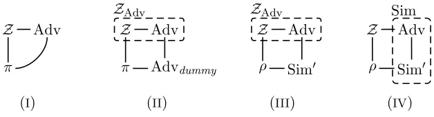
Figure 1: Completeness of the dummy-adversary: proof steps

Thus, if we writeπ quantum-UC-emulatesF, we mean thatπ quantum-UC-emulatesρ_F

whereρ_F consists of the functionalityF and the dummy-parties corresponding to the parties inπ. More precisely:

Definition 7 Let π be a protocol and F be a functionality. We say that π quantum-UC-emulatesF if π quantum-UC-emulates ρ_F where ρ_F :={P˜ :P ∈parties_π} ∪ {F}.

2.5 Dummy-adversary

In the definition of UC-security, we have three entities interacting with the protocol: the adversary, the simulator, and the environment. Both the adversary and the environment are all-quantified, hence we would expect that they do, in some sense, work together. This intu-ition is backed by the following fact which was first noted by Canetti [Can01]: Without loss of generality, we can assume an adversary that is completely controlled by the environment. This so-called dummy-adversary only forwards messages between the environment and the protocol. The actual attack is then executed by the environment.

Definition 8 (Dummy-adversary Advdummy) When activated, the dummy-adversary

Advdummy measures Hclass; call the outcome m. If m is of the form (environment,

adversary, m′₎_{, initialize} _Hclass _with _m_′_. _{Otherwise initialize} _Hclass _with ₍_adversary_,

environment, m). In all cases, the quantum communication register is not modified (i.e., the message in that register is forwarded).

Lemma 9 (Completeness of the dummy-adversary) Assume that π (a, s) -BQS-UC-emulates ρ with respect to the dummy-adversary (i.e., instead of quantifying over all ad-versaries Adv, we fix Adv := Advdummy). Then π (a, s)-UC-emulatesρ.

Proof of Lemma 9. In [Unr10], an analogous theorem has been shown for quantum-UC-security. Our proof is essentially the same, except that we additionally have to check that the machines we construct satisfy the required memory bounds.

Assume that π (a, s)-BQS-UC-emulates ρ with respect to the dummy-adversary. Fix an adversary Adv. We have to show that there exists a simulator Sim with QM(Sim) ≤

s+ QM(Adv) such that for all environments Z with QM(Z) + QM(Adv) ≤ a we have that π∪ {Adv,Z} and ρ∪ {Sim,Z} are negligible-close. Furthermore, if Adv is quantum-polynomial-time, Sim has to be quantum-quantum-polynomial-time, too.

For a given environment Z with QM(Z) + QM(Adv)≤a, we construct an environment

ZAdv that is supposed to interact with Advdummy and internally simulatesZ and Adv, and

that routes all messages sent by the simulated Adv to π through Advdummy and vice versa.

Then π∪ {Adv,Z}and π∪ {Advdummy,ZAdv}are perfectly close. (Cf. networks (I) and (II)

(11)

By definition of Advdummy, we have QM(Advdummy) = 0. And by construction of

ZAdv, we have QM(ZAdv) = QM(Z) + QM(Adv). Thus QM(Z) + QM(Advdummy) ≤

QM(Z) + QM(Adv) ≤ a. Since π (a, s)-BQS-UC-emulates ρ with respect to the dummy-adversary, we have that π∪ {Advdummy,ZAdv} and ρ∪ {Sim′,ZAdv} are negligible-close for

some Sim′ with QM(Sim′) ≤ s+ QM(Advdummy) and all Z. (Cf. networks (II) and (III).)

Since Advdummy is quantum-polynomial-time, so is Sim′. We construct a machine Sim that

internally simulates Sim′ and Adv (network (IV)). Then ρ∪ {Sim′,ZAdv} and ρ∪ {Sim,Z}

are perfectly close. Summarizing, π∪ {Adv,Z} and ρ∪ {Sim,Z} are negligible-close for all environments Z. Furthermore, since Sim′ is quantum-polynomial-time, we have that Sim is quantum-polynomial-time if Adv is. And QM(Sim′) = QM(Sim) + QM(Adv) ≤

s+ QM(Advdummy) + QM(Adv) =s+ QM(Adv). Thus π (a, s)-BQS-UC-emulates ρ.

Using Lemma 9, we can now prove the deferred Lemma 4 (iv).

Proof of Lemma 4(iv). If the π (∞, s)-BQS-UC-emulates ρ, then π trivially quantum-UC-emulatesρ (the condition QM(Z) + QM(Adv)≤ ∞is trivially fulfilled).

Assume thatπquantum-UC-emulatesρ. Then there is a simulator Sim such that for any environmentZ, π∪ {Advdummy,Z} and ρ∪ {Sim,Z} are negligible-close. Since Advdummy

is quantum-polynomial-time, so is Sim. Lets be a polynomial upper-bound on the running time of Sim. Then QM(Sim) ≤ s. Thusπ (∞, s)-BQS-UC-emulates ρ with respect to the dummy-adversary. By Lemma 9,π (∞, s)-BQS-UC-emulates ρ.

2.6 Composition

For some protocolσ, and some protocolπ, byσπ we denote the protocol whereσ invokes (up to polynomially many) instances of π. That is, in σπ the machines from σ and from π run together in one network, and the machines fromσ access the inputs and outputs ofπ. (That is,σplays the role of the environment from the point of view ofπ. In particular,Z then talks only to σ and not to the subprotocol π directly.) A typical situation would be that σF is some protocol that makes use of some ideal functionalityF, say a commitment functionality, and thenσπ _{would be the protocol resulting from implementing that functionality with some}

protocolπ, say a commitment protocol. One would hope that such an implementation results in a secure protocol σπ. That is, we hope that if π BQS-UC-emulates F and σF BQS-UC-emulates G, then σπ _{BQS-UC-emulates} _G_{. Fortunately, this is the case, as long as we pick}

the memory bounds in the right way:

Theorem 10 (Composition Theorem) Let π,ρ, andσ be quantum-polynomial-time pro-tocols. Assume thatσ invokes at most nsubprotocol instances (nmay depend on the security parameter). Assume thatπ (a, s)-BQS-UC-emulatesρ. Then σπ ₍_a₋_QM(_σ₎₋₍_n₋₁₎_{b, ns}₎

-BQS-UC-emulates σρ _where _b_{:= max}_{_QM(_π₎_,_QM(_ρ_{) +}_s_}_.

Proof of Theorem 10. In [Unr10], an analogous theorem has been shown for quantum-UC-security. Our proof is essentially the same, except that we additionally have to check that the machines we construct satisfy the required memory bounds.

Sinceσis quantum-polynomial-time,σinvokes at most a polynomial number of instances of its subprotocolπorρ. We can thus assume thatnis polynomially-bounded. Sinceπ(a, s )-BQS-UC-emulatesρ, there is a quantum-polynomial-time simulator Sim′ with QM(Sim′)≤s

such that for all environmentsZ with QM(Z) = QM(Z) + QM(Advdummy)≤awe have that

π∪ {Advdummy,Z} andρ∪ {Sim′,Z} are negligible-close. In the following, we call Sim′ the

(12)

(I)

Z

Adv

σ π_..1

.

πn

(II)

Z

Adv

σ

Sim′₁ ρ1

..

. ... Sim′_n ρn

Sim

(III)

Z

Adv

σ

π1

.. .

πi−1

Advdummy πi

Sim′_i+1 ρi+1

..

. ... Sim′_n ρn

Zσ,i

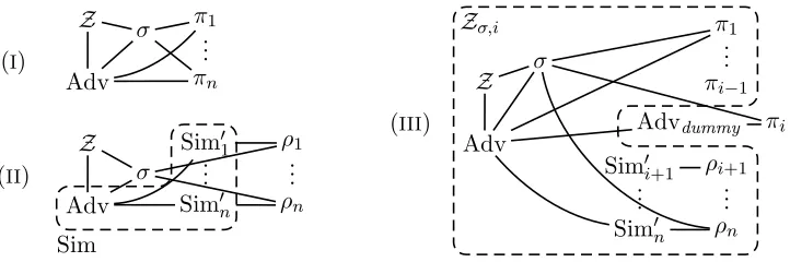
Figure 2: Networks occurring in the proof sketch of Theorem 10. Network (I) represents the real model, (II) the ideal model, and (III) the hybrid case. To avoid cluttering, in (III), the connections toπi−1, Sim′i+1, and ρi+1 have been omitted.

Let a quantum-polynomial-time adversary Adv be given (that is supposed to attack σπ). We construct a simulator Sim that internally simulates the adversary Adv and ninstances Sim′₁, . . . ,Sim′_nof the dummy-simulator Sim′. The simulated adversary Adv is connected to the environment and to the protocolσ, but all messages between Adv and thei-th instanceπi

of π are routed through the dummy-simulator-instance Sim′_i (which is then supposed to transform these messages into a form suitable for instances of ρ). The simulator Sim is depicted by the dashed box in network (II) in Figure 2. We have QM(Sim)≤ns.

We have to show that for any environmentZ with QM(Z) + QM(Adv)≤a−QM(σ)−

(n−1)bwe have thatσπ_{∪ {}_Adv_,_Z}_and _σρ_{∪ {}_Sim_,_Z} _{are negligible-close (networks (}_I_{) and}

(II) in Figure 2).

For this, we construct a hybrid environment Zσ,i. (Zσ,i is depicted as the dashed box in

network (III) in Figure 2.) This environment internally simulates the machines Z, Adv, the

protocol σ, instances π1, . . . , πi−1 of the real protocolπ, and instances Sim′i+1, . . . ,Sim′n and

ρi+1, . . . , ρn of the dummy-simulator Sim′ and the ideal protocol ρ, respectively. The

com-munication between Z, Adv, andσ is directly forwarded by Zσ,i. Communication between

Adv and the j-th protocol instance is forwarded as follows: If j < i, the communication is simply forwarded to πj. If j > i, the communication is routed through the corresponding

dummy-simulator Sim′_j (which is then supposed to transform these messages into a form suit-able for ρj). And finally, if j =i, the communication is passed to the adversary/simulator

outside of Zσ,i. Communication betweenσ and the instances ofπ orρ is directly forwarded.

SinceZσ,iinternally simulates one copy ofZ, one copy of Adv, one copy ofσ,i−1 copies

ofπ, and n−icopies of Sim′ and ρ. Thus

QM(Zσ,i) = QM(Z) + QM(Adv) + QM(σ) + (i−1)QM(π) + (n−i)(QM(Sim′) + QM(ρ))

≤a−QM(σ)−(n−1)b+ QM(σ) + (i−1)QM(π) + (n−i)(QM(Sim′) + QM(ρ))

≤a−QM(σ)−(n−1)b+ QM(σ) + (i−1)b+ (n−i)b=a.

We will now show that there is a negligible function µ such that

|Pr[Exec_π_∪{_Adv_dummy_,_Z_σ,i_}(k, z) = 1] − Pr[Exec_ρ_∪{_Sim′_,

Zσ,i}(k, z) = 1]| ≤ µ(k) for any

security parameterkand any i= 1, . . . , n. For this, we construct an environmentZσ which

expects as its initial input a pair (i, z), and then runsZσ,iwith inputz. Since QM(Zσ,i)≤a,

we have QM(Zσ) ≤a. Since π∪ {Advdummy,Z} and ρ∪ {Sim′,Z} are negligible-close for

all quantum-polynomial-time environments Z with QM(Z) ≤ a, π∪ {Advdummy,Zσ} and

(13)

difference of Pr[Exec_π_∪{_Adv_dummy_,_Z_σ,i_}(k, z) = 1] = Pr[Exec_π_∪{_Adv_dummy_,_Z_σ_}(k,(i, z)) = 1] and Pr[Exec_ρ_∪{_Sim′_,

Zσ,i}(k, z) = 1] = Pr[Execρ∪{Sim′,Zσ}(k,(i, z)) = 1] is bounded by µ(k) for

alli, k, z.

The game Exec_π_∪{_Adv_dummy_,_Z_σ,i_}(k, z) is depicted as network (III) in Figure 2 (except that we wroteπiinstead ofπ). Observe that Execρ∪{Sim′

,Zσ,i+1}(k, z) (note the changed indexi+1)

contains the same machines as Execπ∪{Advdummy,Zσ,i}(k, z) (when unfolding the simulation

performed byZσ,iinto individual machines) except for the difference that the communication

with thei-th instance ofπ is routed through the dummy-adversary Advdummy. However, the

latter just forwards messages, so π∪ {Advdummy,Zσ,i} and ρ∪ {Sim′,Zσ,i+1} are perfectly

close.

Using the triangle inequality, it follows that |Pr[Exec_π_∪{_Adv_dummy_,_Z_σ,n_}(k, z) = 1] −

Pr[Exec_ρ_∪{_Sim′

,Zσ,1}(k, z) = 1]| is bounded by n · µ(k) which is negligible. Moreover,

Exec_π_∪{_Adv_dummy_,_Z_σ,n_}(k, z) and Exec_σπ_∪{_Adv,_Z}(k, z) describe the same game (up to

unfold-ing of simulated submachines and up to one instance of the dummy-adversary). Similarly, Exec_ρ_∪{_Sim′

,Zσ,1}(k, z) and Execσρ∪{Sim,Z}(k, z) describe the same game (up to unfolding of

simulated submachines). Thus

Pr[Exec_σπ_∪{_Adv,_Z}(k, z) = 1]−Pr[Exec_σρ_∪{_Sim,_Z}(k, z) = 1]

is negligible and thus σπ ∪ {Adv,Z} and σρ∪ {Sim,Z} are negligible-close. Furthermore, since Sim′ is quantum-polynomial-time, we have that Sim is quantum-polynomial-time if Adv is. As mentioned above, QM(Sim)≤ns.

Since this holds for all Z with QM(Z) + QM(Adv) ≤ a−QM(σ)−(n−1)b, and the construction of Sim does not depend onZ, we have thatσπ (a−QM(σ)−(n−1)b, ns

)-BQS-UC-emulatesσρ_.

Theorem 11 (Composition Theorem) Let π and σ be quantum-polynomial-time proto-cols and F and G be quantum-polynomial-time functionalities. Assume that σ invokes at most one subprotocol instance. Assume that π (a, s)-BQS-UC-emulates F and that σF (a−QM(σ) +s, s′)-BQS-UC-emulatesG. Then σπ (a−QM(σ), s+s′)-BQS-UC-emulatesG.

The proof of this theorem is very similar to that in [Unr10], except that we have to keep track of the quantum memory used by various machines constructed in the proof.

Proof. From Theorem 10, withn= 1, we get thatσπ (a−QM(σ), s)-BQS-UC-emulates σF. By assumption,σF ₍_a₋_QM(_σ_{) +}_{s, s}′_{)-BQS-UC-emulates}_G_{. By transitivity (Lemma 4 (ii)),} we get that σπ (a−QM(σ), s+s′)-BQS-UC-emulates G.

Notice that in the composition theorem (Theorem 11), the outer protocol σ is only al-lowed to invoke one instance of the subprotocol π. This stands in contrast to the univer-sal composition theorem for classical-UC [Can01] and for quantum-UC [Unr10] where any polynomially-bounded number of concurrent instances ofπis allowed. In fact, this is not just a limitation of our proof technique.11 _{For example, assume a protocol}_πA→B

COM that (a, s

)-BQS-UC-emulates the commitment functionality FA→B

COM with sender Aand recipient B. Assume

further that π_COMA→B does not use any functionalities as setup. As we will see later, such a protocol exists. Now let π_COMB→A be the protocol that results from exchanging the roles of A

and B. ThenπB→A

COM (a, s)-BQS-UC-emulates FCOMB→A. Consider the concurrent composition

of πA_COM→B and π_COMB→A. In this protocol, a corrupted Bob may reroute all messages between the Alice in the first protocol and Alice in the second protocol. Thus, if Alice commits to a

11_{In the proof, the difficulty arises from a hybrid argument where the protocol}_π_{is executed together in one}

(14)

random valuev in the first protocol, Bob commits to the same valuevin the second protocol without knowing it. It is easy to see that in a concurrent composition of FA→B

COM andFCOMB→A,

this is not possible. Thus the composition of π_COMA→B and π_COMB→A does not (a′, s′ )-BQS-UC-emulate the composition ofF_COMA→BandF_COMB→A(for any parametersa′, s′). To convert this into an example of a protocol that does not even compose with itself, just consider the protocol

π_COMA↔B in which Bob may choose whetherF_COMA→B or F_COMB→A should be executed. It might be possible to makeπA_COM↔Bself-composable by adding suitable tags inside the messages, but the definition of BQS-UC-security does not enforce this.

Although BQS-UC-security does not guarantee for concurrent self-composability, individ-ual protocols may have this property. In order to formulate this, we introduce the concept of the multi-session variant of a protocol. Given a protocol π and a polynomially-bounded

n, we defineπn to be the protocol that executes ninstances of π concurrently. Then, from Theorem 11, we immediately get the following corollary:

Corollary 12 Let π and σ be quantum-polynomial-time protocols andF andG be quantum-polynomial-time functionalities. Letn, m≥0 be integers (depending on the security parame-ter). Assume that σ invokes at mostm subprotocol instances. Assume that πnm ₍_{a, s}₎

-BQS-UC-emulates Fnm and that (σF)n (a−nQM(σ) +s, s′)-BQS-UC-emulates Gn. Then (σπ)n (a−nQM(σ), s+s′₎_{-BQS-UC-emulates} _Gn_.

2.7 Quantum lifting

In [Unr10], it has been shown that for classical protocols, classical-UC-security implies quantum-UC-security (quantum lifting theorem). This theorem is very useful when reusing results from the classical-UC setting: For example, if a classical protocol σF classical-UC-emulates a functionality G, and a quantum protocol π quantum-UC-emulates F, then the quantum lifting theorem gives us thatσF quantum-UC-emulatesG, and then by the compo-sition theoremσπ _{quantum-UC-emulates}_G_.

A similar result also holds for BQS-UC:

Theorem 13 (Quantum lifting) If π and ρ are classical protocols and π classical-UC-emulatesρ, then π (∞,0)-BQS-UC emulates ρ.

Proof. In [Unr10], an analogous theorem has been shown for quantum-UC-security. Our proof is essentially the same, except that we additionally have to check that the simulator Sim we construct has QM(Sim) = 0. However, since Sim is a classical machine, this is trivial.

Given a machine M, let C(M) denote the machine which behaves like M, but measures incoming messages in the computational basis before processing them, and measures outgoing messages in the computational basis. More precisely, the superoperator E_C(k)_(M) first invokes

Eclass on Hclass ⊗ Hquant, then invokes EM(k) on Hstate ⊗ Hclass ⊗ Hquant, and then again

invokesEclass on Hclass⊗ Hquant. Since it is possible to simulate quantum Turing machines

on classical Turing machines (with an exponential overhead), for every machine M, there exists a classical machineM′ _{such that}_C₍_M_{) and}_M′ _{are perfectly indistinguishable.}12

We define the classical dummy-adversary Advclass

dummy to be the classical machine that is

defined like Advdummy (Definition 8), except that in each invocation, it first measuresHclass,

Hquant_{, and}_Hstate _{in the computational basis (i.e., it applies}_E

class toHstate⊗Hclass⊗Hquant)

and then proceeds as does Advdummy. Note that Advclassdummy is probabilistic-polynomial-time.

(15)

By Lemma 9, we only need to show that for any setC of corrupted parties, there exists a quantum-polynomial-time machine Sim with QM(Sim)≤0 + QM(Advdummy) = 0 such that

for every machineZ, the real model πC∪ {Z,Advdummy}and the ideal modelρC∪ {Z,Sim}

are negligible-close.

The protocol π is classical, thus πC _{is classical, too, and thus all messages forwarded}

by Advdummy from πC to Z have been measured in the computational basis by πC, and

all messages forwarded by Advdummy from Z to πC will be measured by πC before being

used. Thus, if Adv would additionally measure all messages it forwards in the computa-tional basis, the view ofZ would not be modified. More formally, πC∪ {Z,Advdummy} and

πC∪ {Z,Advclass_dummy}are perfectly close. Furthermore, since bothπC and Advclass_dummy measure all messages upon sending and receiving,πC _{∪ {Z}_,_Advclass

dummy}and πC ∪ {C(Z),Advclassdummy}

are perfectly close. Since it is possible to simulate quantum machines on classical machines (with an exponential overhead), there exists a classical machineZ′ that is perfectly

indistin-guishable fromC(Z). ThenπC ∪ {C(Z),Advclass_dummy}and πC ∪ {Z′,Advclass_dummy}are perfectly close. Since Advclass_dummy and Z′ are classical and Advclass_dummy is polynomial-time, there exists a classical probabilistic-polynomial-time simulator Sim (whose construction is independent of

Z′) such thatπC∪ {Z′,Adv_dummyclass } and ρC ∪ {Z′,Sim} are negligible-close.

ThenρC∪ {Z′,Sim}andρC∪ {C(Z),Sim}are perfectly close by construction ofZ′. And since both ρC _{and Sim measure all messages they send and receive,} _ρC _{∪ {C}₍_Z₎_,_Sim_} _and

ρC∪ {Z,Sim} are perfectly close.

Summarizing, we have thatπC∪{Z,Advdummy}andρC∪{Z,Sim}are negligible-close for

all environments Z. Furthermore, Sim is classical probabilistic-polynomial-time and hence quantum-polynomial-time and its construction does not depend on the choice of Z. And since Sim is classical, QM(Sim) = 0. Thusπ (∞,0)-BQS-UC-emulates ρ.

3 Commitments

3.1 Extractable commitments

In this section, we present the notion of online-extractable commitments in the BQS model. These will be used as a building block for constructing BQS-UC commitments in the next section.

Definition 14 ((ε, a)-BQS-hiding) Given a commitment protocol π with sender Alice and recipient Bob, and an adversary B′ corrupting Bob, we denote withhA(m), B′iB′ the output

of B′ in an interaction between Alice and B′ where Alice commits to m.

We call π (ε, a)-BQS-hiding iff for all a-memory bounded B′ _{and all} _m₁_{, m}₂ _∈ _M_{, we}

have that Pr[hA(m₁), B′i_B′ = 1]−Pr[hA(m₂), B′i_B′ = 1]

≤ε. HereM is the message space

of the commitment scheme.

(16)

Parameters: Integern(the length of the transmitted string). The parameters may depend on the security parameter k.

Parties: The sender Alice A and the recipient Bob B. Inputs: None.

Protocol:

1. Alice picks a randomx∈ {0,1}n _and _θ_{∈ {}₊_,_×}n_{. Then she encodes and sends each bit}

xi in the basisθi, i.e., she sends|Ψi:=|xiθ to Bob.

2. Bob picks a random ˜θ∈ {0,1}n _{and measures the} _i_{-th qubit of} _|_Ψ_i _{in basis} _θ

i. Call the

outcomes ˜xi.

3. Both parties wait until the quantum memory bound becomes effective.13 4. Alice sendsθ to Bob and outputsx.

5. Bob computesI :={i:θi = ˜θi} and outputs (I,x˜I).

Figure 3: Weak string erasure protocol πWSE from [KWW09].

Definition 15 ((ε, s)-online-extractable) Given a commitment protocolπwith sender Al-ice and recipient Bob, an extractor is a machine BS that, after the commit phase, gives an

outputV′ _{and then executes the (honest) code of Bob for the open phase and outputs a value}

V (the accepted value). (In particular, BS needs to provide an initial state for the program

of the open phase of Bob that matches the interaction so far.) We write V =⊥ if the open phase fails.

For an adversary A′, we denote with hA′, BiA′ (hA′, B_Si_A′) the output of A′ in an

inter-action betweenA′ and Bob (BS) whereA′ is givenV after Bob (BS) terminates.

We call π (ε, s)-online-extractable iff there exists an s-memory bounded quantum-polynomial-time extractor BS such that for all adversaries A′, we have that

Pr[hA′, Bi_A′ = 1]−Pr[hA′, BSiA′ = 1] ≤εand in an interaction ofA′ andB_S, we havePr[V /∈ {V′,⊥}]≤ε.

Constructing online-extractable commitments. K¨onig, Wehner, and Wullschleger [KWW09] present a commitment scheme in a generalization of the bounded quantum stor-age model. Although they only show that it is hiding and binding, their scheme turns out to be also online-extractable. Their construction proceeds in two steps. First, they give a protocol for what they call aweak string erasure (WSE). A WSE is a protocol between Alice and Bob after which Alice outputs a bitstring X and Bob outputs a set of indices I and the bitstringX_I consisting of X restricted to the indices I. The properties guaranteed by a weak string erasure are – informally – that Bob does not learn too much aboutX_I∁, and that Alice has no information about I. From a WSE, we can construct a commitment scheme as follows: If Alice wishes to commit to a string m, Alice and Bob perform a WSE. Then Alice sendsm⊕F(X) to Bob whereF is a universal hash function with suitable parameters. Furthermore, Alice sendsS(X), the syndrome ofX under a suitable linear code. Since Bob only learns X_I, S(X), and little about X_I∁, the string X has high min-entropy from Bob’s point of view. ThusF(X) looks random to Bob and the commitment is hiding. To open the commitment, Alice sendsX. Since she does not knowI, Alice will be detected if she sends an ˆX that is substantially different from X. If Alice sends an ˆX that differs fromX only at a few indices, the syndromesS(X) and S( ˆX) will not match. Thus Alice is forced to send

ˆ

X=X; the commitment is binding. The precise protocols are given in Figures 3 and 4.

13_{Formally, in our model this step does not exist because our model assumes that the quantum memory}

(17)

Parameters: Integers ℓ(the length of the committed value),n < ℓ, andκ, d≤n. A binary (n, κ, d)-linear code whereS(ω)∈ {0,1}n−κ denotes the syndrome of a codewordω∈ {0,1}n. A familyFof universal hash functionsF :{0,1}n_{→ {}₀_,₁_}ℓ_{. All parameters may depend on}

the security parameterk.

Subprotocols: Then-bit WSE protocol from Figure 3. Parties: The sender Alice A and the recipient Bob B.

Inputs: In the commit phase, Alice getsv withv ∈ {0,1}ℓ. Bob gets no inputs. Commit phase:

C1. Alice and Bob execute the WSE protocol. Alice gets x, Bob gets I andx_I.

C2. Alice picks a hash function F ← F, computes p := v⊕F(x), computes the syndrome

σ:=S(x), and sends (F, σ, p) to Bob. Open phase:

O1. Alice sends ˆx:=x to Bob.

O2. Bob checks whetherσ =S(ˆx) and ˆx_I =x_I. Otherwise, Bob aborts.

O3. Bob computes v:=p⊕F(ˆx) and outputs v. (I.e., Bob accepts the opened value v.)

Figure 4: Commitment schemeπKWW from [KWW09].

The hiding property of πKWW has already been proven in [KWW09], we only need to

specialize their result to the BQS model.

Lemma 16 Fix constants δ, ν > 0 with δ+ν < 1₂. Fix some integer a (the adversary’s memory bound; dependent on the security parameter k). Assume that a ≤ νn and n ≥ k. Assume that ℓ≤ 1₂n−δn−νn−(n−κ)−k. (n, κ, ℓ refer to the parameters in Figure 4.) Then there is an exponentially-small ε >0 such that πKWW is (ε, a)-BQS-hiding.

Proof. In [KWW09], the notion of an (n, λ, ε′_{)-WSE protocol is introduced. Here} _n _{is the} length of the transmitted string, and λn lower bounds the knowledge that Bob has about the string (in terms of min-entropy, and up to an error probabilityε′). The precise definition is given in [KWW09]; for the present proof we will not need any details. Their definition is parametrized by an operator F that describes the evolution of the quantum state in Bob’s memory. To model the special case of the BQS model in which the adversary’s memory has a qubits, we have to choose F to be the identity on a-qubit states. Let PF

succ(n′) :=

max(Dx)x,(ρx)x

1 2n′

P

x∈{0,1}n′tr D_xF(ρ_x)where (D_x)_xgoes over all POVMs (measurements), and (ρx)xover all families ofa-qubit mixed states. Intuitively,PsuccF (n′) denotes the maximum

probability of correctly decoding a randomn′-bit string after it has been stored in anaqubit state. In [KW09, page 1] it is shown that PF

succ(n′) ≤2−n

′

(R−1) _{= 2}−a+n′

for R := _na′. By [KWW09, Theorem 3.2], for any constant δ ∈ (0,1₂), we have that πWSE is an (n, λ, ε′

)-WSE protocol where λ = −1_nlogPsuccF (1₂ −δ)n

and ε′ = 2e− nδ2

512(4+log 1_δ)2_{. We have that}

λ ≥ −_n1 log 2−a+(12−δ)n = (1

2 −δ)− na ≥ 12 −δ −ν. Let ε′′ := max{2−k/2, ε′}. Since

πWSE is an (n, λ, ε′)-WSE protocol it is also an (n, λ, ε′′)-WSE protocol. Furthermore, ℓ≤

λn−(n−κ)−2 log 1/ε′′. Then, by [KWW09, Lemma 4.3],14 if πWSE is an (n, λ, ε′′)-WSE

protocol, then πKWW is (ε, a)-BQS-hiding with ε:= 3ε′′.15 Since δ is constant and n ≥ k,

14_{Strictly speaking, [KWW09, Lemma 4.3] analyzes a protocol that commits to a random value (and in}

particular does not send the valuepin the commit phase). It is, however, straightforward to see that their proof also applies toπKWW as presented in Figure 4.

15_{The definition of hiding is formulated slightly differently in [KWW09] but can easily be seen to imply our}

(18)

we have thatε′ and hence also ε= 3 max{2−k/2, ε′} is exponentially-small.

We proceed to show that πKWW is online-extractable. Since K¨onig et. only showed the

binding property, we need to extend the proof of [KWW09]. The main ideas are, however, already present in [KWW09]. Intuitively, online-extractability ofπKWW is not surprising: If

Bob has an unbounded amount of quantum memory, he can delay the measurement of the qubits in πWSE and thus get all the bits xi. That is, πWSE is online-extractable. Then, in

πKWW, Bob will know x already in the commit phase and can thus compute v =p⊕F(x)

(after error-correcting x to match the syndrome σ). Since v is the committed value, this implies thatπKWW is online-extractable. To make this argument formal, we need to ensure

that even if Alice cheats, she is not able to send some ˆxin the open phase which differs from the valuex that Bob extracted. The proof of this fact is similar to the proof of the binding property in [KWW09].

We begin by making the fact formal that Bob (given sufficient quantum memory) can extract in πWSE.

Definition 17 (Online-extractable WSE) A n-bit WSE protocol π consisting of sender AWSE _{and recipient} _BWSE _is _s_{-online-extractable} _{if there exists an} _s_{-memory bounded} quantum-polynomial-time machine BWSE

S with the following properties:

• BWSE

S outputs an n-bit string x.

• For any adversary A′, let ρA′_B denote the state of A′ after interacting with BWSE.

Here A′ _{gets the outputs} _x

I and I made by BWSE. Let σA′_I_Xˆ

I denote the state of A ′

after interacting with BWSE

S . Here A′ gets xI and I where x is the output of BWSES

and I is a uniformly random subset of {1, . . . , n}.16 ThenρA′_B =σ

A′ IXˆI.

Note that in this definition, we do not require the extractor BWSE

S to produce the set I.

Instead, in an execution of A′ and BWSE

S , we choose I randomly. Alternatively, we could

also letBWSE

S pick I and require thatI is uniformly random and independent ofx and the

state ofA′_{; this would lead to an equivalent definition.}

The definition could be generalized by allowing an error ε; we would then require that the trace distance εbetweenρA′_B and σ

A′_I_Xˆ

I is bounded by ε. For our purposes, however, the present definition is sufficient.

Lemma 18 (Online-extractability of πWSE) πWSEisn-online-extractable. (Herenis as

in Figure 3.)

[KWW09, Theorem 3.5] states a weaker property (called “security for Bob”). The proof of that theorem, however, explicitly constructs a simulator and proves the properties required by Definition 17. Thus, their proof also constitutes a proof for our Lemma 18.

Given an online-extractable WSE protocol, we get an online-extractable commitment scheme:

Lemma 19 Assume that the code with syndrome S has efficient error-correction. If πWSE

is an s-online-extractable WSE protocol for some s, then πKWW is an (s,2−d/2)

-online-extractable commitment scheme. Hered,S are the parameters from Figure 4. Notice that we do not require that πWSE is the protocol from Figure 3.

Proof. To show that πKWW is online-extractable, we first construct the extractor BS. BS

follows the program of Bob (Figure 4), except that in Step C1, Bob runs the extractor

16_{The names of the states}_ρ

(19)

BWSE

S from Definition 17 (which yields an n-bit string x), chooses a random subset I of

{1, . . . , n}, and computesx_I. In all other protocol steps, BS behaves like Bob in Figure 4.

After the commit phase, BS computes an x∗ with Hamming distance ω(x, x∗) ≤ (d−1)/2

and S(x∗) = σ. (This can be done in polynomial-time since the code with syndromeS has efficient error-correction.) ThenBS computesv′ :=p⊕F(x∗) and outputsv′. (If nox∗ with

ω(x, x∗)≤(d−1)/2 exists, thenBS sets v′:=⊥ instead.)

Since BWSE

S satisfies Definition 17, we have that Pr[hA′, BiA′ = 1] = Pr[hA′, B_Si_A′ = 1]. To show that πKWW is (s,2−d/2)-online-extractable, we thus are left to show that Pfail :=

Pr[v /∈ {v′,⊥}]≤2−d/2.

From the construction ofπKWW, we have thatPfail is upper bounded by the probability

that ˆx 6=x∗ _and _S(ˆ_x_{) =}_σ _{and ˆ}_x

I =xI. Fix some ˆx, x∗ with ˆx 6=x∗ and S(ˆx) =σ. From S(ˆx) =σ =S(x∗) we haveS(ˆx−x∗) = 0. Hence ˆx−x∗has Hamming-weight at leastd. Thus

ω(ˆx, x∗)≥d. Sinceω(x, x∗)≤(d−1)/2, it follows that ω(x,xˆ)≥d−(d−1)/2≥d/2. (In the case wherev′ ₌_⊥_{, we have}_ω₍_{x, x}∗₎_>₍_d₋₁₎_/_{2 for all} _x∗ _{and hence}_ω₍_x,_x_ˆ₎_>₍_d₋₁₎_/₂ and hence ω(x,xˆ) ≥ d/2.) Since I is chosen independently of x,xˆ, and each iis in I with probability 1₂, it follows that x_I = ˆx_I with probability at most (1₂)ω(x,ˆx) ≤ 2−d/2. Thus

Pfail ≤2−d/2.

Combining our results on πWSEand πKWW, we get the following theorem:

Theorem 20 (Online-extractable commitments) For any polynomially-bounded inte-gers a and ℓ, there is a constant-round 0-memory bounded (ε, a)-BQS-hiding (ε, s) -online-extractable commitment scheme π for some exponentially-small ε and some polynomially-bounded s. The message space of π isM ={0,1}ℓ_.

Proof. Reed-Solomon codes [RS60] are (2b −1,2b−d, d)-linear codes over GF(2b) (for any

b, d). By representing each symbol as a b-bit string, they can be converted into binary ((2b₋₁₎_b,₍₂b₋_d₎_{b, d}_{)-linear codes. Error-correction is efficiently possible using the}

Berlekamp-Massey algorithm [Ber67, Ber84].

Let δ, ν > 0 be some constants with δ+ν < 1₂. (E.g., δ = ν = 1₆.) Let k denote the security parameter. All values introduced below will depend on k. Letd:=k. Letb be the smallest integer such thatn:= (2b−1)bsatisfies 1₂n−δn−νn−(d−1)b−k≥ℓand νn≥a

and n ≥k. Such a b exists and then n is polynomially-bounded. Let κ := (2b−d)b. Let S be the syndrome of the (n, κ, d)-Reed-Solomon code. LetF be a family of universal hash functions F :{0,1}n → {0,1}ℓ. Such functions exist for anyn, ℓ; for example, the set of all affine transformations from{0,1}n to {0,1}ℓ is easily seen to be strongly universal.

Since ℓ≤ 1₂n−δn−νn−(d−1)b−k= 1₂n−δn−νn−(n−κ)−d, by Lemma 16, we have thatπKWW is (ε1, a)-BQS-hiding for some exponentially-smallε1.

And with s:=n, by Lemmas 18 and 19, we get that πKWW is (s, ε2)-online-extractable

with ε:= 2d/2_.

Since both ε1 and ε2 are exponentially-small, the theorem holds with ε:= max{ε1, ε2}.

3.2 BQS-UC commitments

In this section, we present a commitment schemeπCOM that is BQS-UC-secure for memory

boundaand for nconcurrent instances of πCOM. The parametersaand ncan be arbitrary,

but πCOM depends on them. To state our result, we first define the ideal functionality for

Concurrent composition in the bounded quantum storage model

Concurrent composition in the

bounded quantum storage model

Contents

1

Introduction

2

Bounded quantum storage UC

3

Commitments