c
Owned by the authors, published by EDP Sciences, 2012
Modified Taylor-tests with miniaturized samples
F. Bagusat and I. Rohr
Fraunhofer Institute for High-Speed Dynamics, Ernst-Mach-Institut, EMI, Eckerstrasse 4, 79104 Freiburg, Germany
Abstract. A reversed Taylor-test with application of a velocity interferometer is in use at EMI, called modified Taylor-test (MTT). The experiment consists of impacting a fixed sample rod and observing the rear side of the sample by a velocity interferometer of the VISAR type. The setup enables to determine high-dynamic material data of the sample by evaluating the measured free surface velocity time curve. Normally, rods with a dimension of 6 mm diameter and 60 mm length have been investigated. Samples with this diameter are not producible from sheets: Sheet steels typically have a maximum diameter of 3 mm. Furthermore, it would be a general advantage to be able to work with small sample sizes when seldom or expensive materials have to be investigated. Therefore, efforts for reducing the sample size for MTTs have been made. In recent tests, Taylor rods of 1.5 mm diameter and a length of 15 mm have been used. VISAR data could be captured from these samples, which are comparable with data from larger-size MTTs. This finding offers new perspectives for high-dynamic testing of materials which only allow the production of small sample diameters.
1 Introduction
1.1 The modified Taylor-test
A reversed Taylor-test combined with a VISAR (veloc-ity interferometer system for any reflector [1–4]) can be used as a method for measuring the elastic-plastic wave processes in impacted rod-shaped samples. In order to dis-tinguish this variant of a Taylor-test from the conventional one [5–7], it is here called modified Taylor-test (MTT). The principle of conduction is easy. The sample Taylor rod is held fixed and impacted by a projectile with sufficiently high velocity. In an elasto-plastic material, the impact generates a plastic as well as an elastic wave within the sample. The rear side of the sample rod is accelerated by the influence of the elastic wave; this can be observed by a VISAR. From the free surface velocity time curve of the VISAR signal, dynamic material properties can be derived. The experiment delivers high-dynamic material data with typical strain rates of 1000 1/s and higher which can supply split Hopkinson bar and planar plate investigations in a suitable manner. Recent details regarding the background of conduction of this type of test and its applications at EMI can be found in the literature [8, 9]. The MTT setup used at EMI has seen several improvements and changes regarding setup details, experimental conduction and data evaluation, which are still being continued. The MTT delivers very valuable data for a simulation of the dynamic material behavior due to the fact that VISAR data are captured continuously during the deformation process of the samples [8, 9]. EMI-related MTTs are typically conducted with a length-(L)-to-diameter-(D) ratio of the samples ofL/D=10 : 1.
Interesting further examples of the usage of an MTT setup conducted in the last decade are investigations of stainless steel, copper, titanium, vanadium and composites (L/D = 4 : 1) [10–12]. For this work, in addition to a VISAR, precise high-speed camera photographs were presented in order to specify the impact-related deforma-tion of the samples. The experiments served as a basis
for comparisons of different constitutive models. Also, a symmetric configuration of an MTT for which a projectile rod is fired onto a target rod is known (investigations of annealed copper, L/D = 10 : 1), where high-speed cameras, a VISAR and strain gauges have been used [13]. All Taylor rod samples used for these experiments [10–13] had diameters in the range between 9 mm and 19 mm.
The MTT can be executed similarly and in addition to planar plate tests.
The main advantages of the MTT in comparison to the conventional Taylor-test are its simplicity in preparation as well as the data evaluation which needs only a VISAR data reduction and an inspection of the VISAR curve, both executable within a few minutes. The usage of a VISAR instead of, e. g., strain gauges [14] reduces the preparation efforts of a sample and is contact-free without mechanical influence on the investigated samples.
1.2 Dynamic data derived from modified Taylor-tests
Basis for the data analysis is that the elastic wave caused by the impact is reflected at the rear side of the sample rod which effects an acceleration of the rear side which can be recorded by the VISAR. Depending on the sample properties, the impact velocity and the properties of the plastic wave in the sample, a step-shaped VISAR free surface velocity time curve can be measured. Due to the limited space in this paper, only formulas for the yield stress, strain and strain rate are repeated [8]. The yield stressYdetermined by the MTT is given by
Y =0.5∗ρ∗c0∗∆uf s
whereρis the density of the Taylor rod sample,c0denotes
the longitudinal velocity of sound and ∆uf s is the height of the (first) velocity step measured with the VISAR at the rear side of the sample. The strainat the yield point can be calculated by
=∆uf s/(2∗c0).
Therefore, the corresponding strain rate is
d/dt=/∆t
where ∆t is the time interval, in which the velocity step ∆uf s takes place. The determination of the ∆uf s and∆t values can be done by the help of mathematical analysis in the specific data interval or, much simpler, graphically depending on the wanted accuracy.
Notes:
(1) The rear side acceleration is only effected by the elastic wave, so the strain and strain rate data are connected with elastic properties. The classical Taylor-test estimates strain, strain rate data and the yield stress according to a plastic deformation.
(2) The aim of this paper isnotto derive and present material data from the investigated samples but to show that a reduction of the geometric dimensions of the sample is possible for material tests.
1.3 The sample size of modified Taylor-tests
The size of the sample rod in EMI-related investigations has normally been 6 mm diameter and 60 mm length, although even larger and smaller samples have been tested; sometimes sample sizes of 5 mm diameter and 50 mm length have been used [9]; also dynamic properties of a tube material with a wall thickness of about 2.5 mm were investigated in analogy to rod-like samples [15].
Taylor rods of 6 mm diameter cannot be produced from sheet steels with a diameter of 3 mm or less. This led to the question if the sample diameter of Taylor rods could be reduced to sizes below 2 mm. From the point of VISAR observation, samples should at least have the diameter of the laser focus, which is about 0.5 mm in our setup. In addition, the VISAR focus should cover a sufficient number of grains of a sample so that signal averaging reduces the statistical variation of the signals of independent experiments [16]. It is also important that the focus will not leave the Taylor rod during the experiment. With a diameter of the Taylor rod larger than the VISAR focus diameter, even these conditions might be met for most sample materials.
A further point is the handling of the samples. This be-gins with the sample preparation, goes on with the surface preparation of the sample (a diffusely reflecting surface should be prepared), continues with the alignment process for the VISAR observation and ends with questions of the stability of the sample holder and the contact of the sample to the sample holder. With increasing diameter of the Taylor rod, all these requirements are easier to fulfill.
Several experiments with C45 Taylor rod samples with a diameter of 1.5 mm and a length of 15 mm were executed, all of them showing the typical stepped free surface velocity time curve of the VISAR signal as known from experiments with aL/Dratio of the samples of 10 : 1.
2 Experimental setup
Samples were prepared from a C45 steel rod of 10 mm diameter. The original material and the produced samples
Fig. 1. Photograph of a Taylor rod with 6 mm diameter and 60 mm length (top) and a miniaturized Taylor rod (1.5 mm diameter and 15 mm length). Both samples were prepared from larger C45 steel rods.
Fig. 2. Photograph of a miniaturized Taylor rod with 1.5 mm diameter in the sample holder setup. Slanted view onto the impacted side of the sample. The second (thinner) object in the sample holder is the impact trigger pin with which the data recording is triggered.
have the same axis orientation. A diameter of 1.5 mm and a length of 15 mm for the miniaturized samples have been chosen. This is probably not the smallest possible size but much smaller compared with the 6 mm by 60 mm sample and represents a compromise between sample size and handling properties.
The miniaturized Taylor rod with 1.5 mm diameter is shown in comparison with a 6 mm diameter Taylor rod in Fig. 1. This figure illustrates the effect of volume reduction reached by the downscaled sample.
The conduction of experiments with these small Taylor rods has been realized very similarly to tests with larger sample sizes. The sample rod is positioned by the help of a polycarbonate mount glued into the sample holder. This piece has a central bore which is a little bit larger than the diameter of the Taylor rod.
Therefore, the Taylor rod is lying in the bore hole, without smooth contact to the polycarbonate mount which suppresses wave transmission in the sample holder. The position of the Taylor rod is fixed in the central bore of the mount by the use of a drop of glue. A prepared sample is shown in Fig. 2.
Table 1.Characteristic data of the experiments.
Exp. Impact Signal Signal
No. velocity quality quality
m/s (pre- (experimental alignment- fringe recording)
before S/N experiment)
S/N
3404 234 3.7:1 4:1
3405 309 11.2:1 1:1 3406 349 15.5:1 7.5:1 3407 264 10:1 >10 : 1
3408 222 2:1 1.2:1
3409 273 5:1 4.3:1
Photomultiplier signals of the fringes were recorded by an oscilloscope of the “Tektronix TDS7104” type with a bandwidth of 1 GHz. The impact chamber was evacuated to a remaining air pressure of about 1 mbar before the experiment. The time interval between the data points presented in the following is 1.6 ns.
3 Experimental results
3.1 Quality of fringe signals
In total, six experiments (numbers 3404 to 3409) with C45 steel samples have been executed. From all experiments, fringe signals were recordable.
In one case (experiment 3407), the diffuse reflection produced a strong signal overshoot on the oscilloscope screen, so that this data set could not be converted into a free surface velocity time curve. The other measurements delivered signals of different quality, see Table 1.
The quality of the VISAR signals can be determined in the pre-alignment procedure just before the experiment by inspecting the fringe signals and estimating their signal-to-noise (S/N) ratios. The signal-signal-to-noise ratio is given by the signal amplitude according to the median signal level in relation to the full noise width of the signal taken from the turn-around regions of the y-t (fringe intensity time) curves.
The VISAR pre-alignment procedure consists of get-ting a nearly perfect circular Lissajous figure, indicaget-ting that the two detector signals of the VISAR have a phase shift of 90 degrees.
The used laser intensity could range from 0.3 W up to 2 W with the 1.5 mm diameter samples. A typical good pre-alignment procedure with samples of 6 mm diameter required laser intensities between 0.2 W and 0.8 W and could reach an S/N value of about 10 : 1 or even better.
In the pre-alignment process, the S/N values are com-parable with typical values reached with rods of 6 mm diameter (experiments 3405 to 3407), but measurements 3404 and 3409 show only about one third or one half of the typical S/N ratio, 3408 even less.
Inspecting the experimental fringe signals, three mea-surements (3404, 3407, 3409) delivered signals for which the S/N was comparable or better than the one observed in
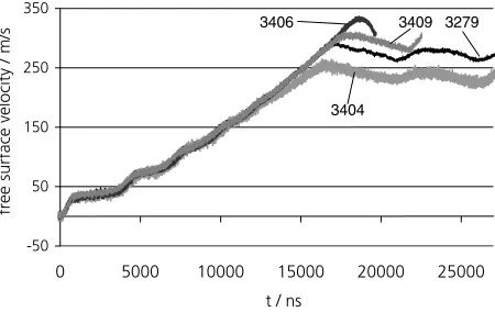
Fig. 3.Free surface velocity time curves of experiments 3404, 3406 and 3409. For comparison, data of the MTT experiment 3279 (with a sample diameter of 6 mm and a length of 60 mm) are plotted in addition. The time scale of data of experiment 3279 has been reduced by division by four.
the pre-alignment process. In two measurements (3406 and 3408), the S/N was reduced by a factor of about two (but one should consider that experiment 3406 delivered the best result of all). Two experiments (3405, 3408) produced only a very weak S/N of about 1 : 1.
The tiny Taylor rods are objects which are difficult to handle. A reduced S/N ratio in the pre-alignment or in the data of some experiments seems to be acceptable.
The polishing of the end surfaces of the samples is known to have a strong influence to the signal’s S/N ratio in the pre-alignment procedure and for the experiment itself. In case of the small Taylor rods, furthermore, the axial alignment of the sample and the stiffness of the sample holder become much more important than for all other high-dynamic material tests conducted with a VISAR.
3.2 VISAR resultswithoutdata smoothing
In experiments 3404, 3406 and 3409, the S/N ratio was 4 : 1 or better (Table 1) so that these data sets could be transformed into the free surface velocity time curve without any data smoothing.
The free surface velocity time curves of these exper-iments are shown in Fig. 3. The shape of the curves is typical, as illustrated by the data of experiment 3279 as a reference. All curves have been shifted in x- and in y-direction so that the signal increases overlap and the zero signals are positioned around the zero level. The curves show a quite well overlap with the reference 3279.
Depending on the different S/N ratio in the fringe signals, the full noise width in the free surface velocity time curves exhibits differences. The signal increase in experiment 3406 did not reach the maximum velocity due to fringe signal loss, therefore, one observes a curve early directed downwards.
3.3 VISAR resultswith datasmoothing
Fig. 4. Effect of data smoothing. Results of experiment 3406 represented by the original data (black) and by the smoothed data (fine white line). The data were smoothed before the data reduction was done.
3409
3404
3406 3279
Fig. 5.Measurement curves of Fig. 3 with data smoothing applied before data reduction for data of experiments 3404, 3406 and 3409. Data of experiment 3279 serve as reference and were not smoothed.
minima and maxima. Attempts have been made to use these data sets directly without any changes for data re-duction. It has been found that this is not possible because the identification of the minima and maxima worked not correctly and produced partially negative velocity intervals in the free surface velocity time curve.
Therefore, all data sets have been smoothed; after that, the data reduction was repeated. The results are presented in this section.
The effect of the data smoothing is illustrated by Fig. 4. It can be seen that the smoothing gives a noise-reduced free surface velocity time curve with the structure of the original data. Relevant velocity changes are maintained.
In Fig. 5, curves already presented in Fig. 3 have been plotted again in the “smoothed version”. The fig-ure demonstrates that the resulting curves of experiments 3404, 3406 and 3409 after data smoothing of the original data look more detailed. Here, for a better identification of the curves, symbols with different sizes have been used.
After data smoothing in the same way as conducted with the data sets of experiments 3404, 3406 and 3409, a successful data reduction could be completed even for experiments 3405 and 3408 which exhibited a very bad S/N ratio. The free surface velocity time curves of these two experiments are shown together with the free surface
3408 3279
3405
Fig. 6.Results of experiments 3405 and 3408 with data smooth-ing applied before data reduction. Data of experiment 3279 serve as reference and were not smoothed.
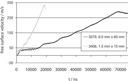
3279, 6.0 mm x 60 mm
3406, 1.5 mm x 15 mm
Fig. 7. Taylor-tests with different sample sizes. Results of ex-periment 3406 (sample of 1.5 mm diameter and 15 mm length) and the reference experiment 3279 (6 mm diameter and 60 mm length). Curves shown with the original time scale.
velocity time curves of the reference data set 3279, see Fig. 6. Despite the fact that they exhibit strong noise, the curves of experiments 3405 and 3408 have the typical shape common for an MTT.
Relevant characteristics describing the dynamical be-havior of the sample material like the first velocity step value and the increase time to this plateau can easily be derived from these curves. Summarizing this, from six experiments executed, five typical free surface velocity time curves were derivable, one curve showed a strong sig-nal overshoot. This means, MTT experiments with small sample dimensions are operable and can deliver dynamical material data.
3.4 Influence of the sample size
In the formula for the yield stress in Sect. 1.2, no direct geometric dependence of the sample size is expressed.
3279, 6.0 mm x 60 mm
3406, 1.5 mm x 15 mm
Fig. 8.Enlargement showing the first third of Fig. 7. The effect of the sample length on the duration of the plateau lengths of the velocity time curve is illustrated.
3279, 6.0 mm x 60 mm
3406, 1.5 mm x 15 mm
Fig. 9.Curves of experiments shown in Fig. 7, but the time scale of experiment 3279 was reduced by multiplying it by 0.25 in accordance with the length ratio of the samples. This operation gives nearly overlapping curves.
3279, 6.0 mm x 60 mm
3406, 1.5 mm x 15 mm
Fig. 10.Enlargement of Fig. 9 showing the region of the first plateau.
For a better illustration of this phenomenon, experi-ments with Taylor rods of different dimensions are shown in Figs. 7 to 10 again. In the first two figures, curves are printed with the original time axis, the last two figures show the same curves but with a scaled time axis. The scaling factors were 0.25 (3279) and 1 (3406) and were chosen in accordance with the length of the sample rods (as already mentioned). It can clearly be seen that the plateau length is a function of the sample length. This should be the case due to the propagation of the elastic wave with constant speed. Furthermore, the slope of the steps of the
free surface velocity time curve depends on the length of the sample. A shorter sample produces a steeper slope representing a higher strain rate. The strain rate increases inversely proportionally to the sample length.
Here, a variation of the strain rate by a factor of four has no significant effect to the measured dynamic yield stress represented by the height of the velocity step.
4 Summary and conclusions
In this investigation, high-dynamic material tests of the MTT type conducted with small Taylor rod samples of 1.5 mm diameter and 15 mm length are presented.
Such small samples enable measurements of dynamic material data concerning flat object pieces like thin plates, sheet steel or wire-like sample material as long as samples can be produced. The negligible material consumption also makes investigations of expensive and seldom materials possible.
The smallness of the sample size requires some efforts in the alignment of the samples for conducting the VISAR experiment. The VISAR focus should cover a statistically representative number of grains. The failure rate of the experiments seems to be comparable to the one executed with larger-size samples.
References
1. L. M. Barker, R. E. Hollenbach, J. Appl. Phys. 43, 4669 (1972)
2. L. M. Barker, K. W. Schuler, J. Appl. Phys.45, 3692 (1974)
3. W. F. Hemsing, Rev. Sci. Instrum.50, 73 (1979) 4. L. M. Barker,Shock Compression of Condensed
Mat-ter 1997, AIP Conference Proceedings CP 429, 833 (1998)
5. G. Taylor, Proc. Royal Soc. London A194, 289 (1948) 6. A. C. Whiffin, Proc. Royal Soc. London A194, 300
(1948)
7. W. E. Carrington, M. L. V. Gayler, Proc. Royal Soc. London A194, 323 (1948)
8. I. Rohr, H. Nahme, K. Thoma, Int. J. Impact Eng.31 401 (2005)
9. I. Rohr, H. Nahme, K. Thoma, C. E. Anderson Jr., Int. J. Impact Eng.35, 811 (2008)
10. D. E. Eakins, N. N. Thadhani, J. Appl. Physics100, 073503 (2006)
11. M. Martin, T. Shen, N. N. Thadhani, Materials Science and Engineering A494, 416 (2008)
12. A. Mishra, M. Martin, N. N. Thadhani, B. K. Kad, E. A. Kenik, M. A. Meyers, Acta Materialia56, 2770 (2008)
13. L. C. Forde, W. G. Proud, S. M. Walley, Proc. Royal Soc. A465, 769 (2009)
14. R. Tham, A. J. Stilp, Journal de Physique49, C3-85 (1988)
15. H. Nahme, EMI Freiburg, Germany, personal commu-nication (2009)