The SABR Model
by Fabrice Douglas Rouahwww.FRouah.com www.Volopta.com
The SABR model is used to model a forward Libor rate, a forward swap rate, a forward index price, or any other forward rate. It is an extension of Black’s model and of the CEV model. The model is not a pure option pricing model— it is a stochastic volatility model. But unlike other stochastic volatility models such as the Heston model, the model does not produce option prices directly. Rather, it produces an estimate of the implied volatility curve, which is subsequently used as an input in Black’s model to price swaptions, caps, and other interest rate derivatives.
1
Process for the Forward Rate
The SABR model of Haganet al. [2] is described by the following 3 equations
dft = tftdWt1 (1)
d t = v tdWt2
E dWt1dWt2 = dt
with initial values f0 and = 0: In these equations, ft is the forward rate, t is the volatility, and Wt1 and Wt2 are correlated Brownian motions, with
correlation . The parameters are
the initial variance
v the volatility of variance
the exponent for the forward rate
the correlation between the Brownian motions.
The case = 0 produces the stochastic normal model, = 1produces the stochastic lognormal model, and = 1
2 produces the stochastic CIR model.
2
SABR Implied Volatility and Option Prices
The prices of European call options in the SABR model are given by Black’s model. For a current forward ratef, strikeK, and implied volatility B the
price of a European call option with maturityT is
with
and analogously for a European put. The volatility parameter B is provided
by the SABR model. With estimates of ; ; v; and ;the implied volatility is
B(K; f) =
Once the parameters ; ; ;andv are estimated, the implied volatility B is a
function only of the forward pricef and the strikeK: Since the SABR model produces implied volatilities for a single maturity, the dependence of B onT
is not re‡ected in the notation B(K; f).
3
Estimating Parameters
The parameter is estimated …rst, and is not very important in the model because the choice of does not greatly a¤ect the shape of the volatility curve. With estimated, there are two possible choices for estimating the remaining parameters
Estimate ; ;and vdirectly, or
Estimate and v directly, and infer from ; v; and the at-the-money volatility, AT M.
3.1
Estimating
From equation (3), the at-the-money volatility AT M is obtained by setting
f =Kin equation (3), which produces
Hence, can be estimated by a linear regression on a time series of logs of ATM volatilities and logs of forward rates. Alternatively, can be chosen from prior beliefs about which model (stochastic normal, lognormal, or CIR) is appropriate. In practice, the choice of has little e¤ect on the resulting shape of the volatility curve produced by the SABR model, so the choice of is not crucial. The choice of , however, can a¤ect the Greeks. Barlett [1] provides more accurate Greeks and shows that they are less sensitive to the choice of :
This is described in Section 5.3.
3.2
First Parameterization–Estimating
; ;
and
v
Once ^ is set, it remains to estimate ; ;andv. This can be accomplished by minimizing the errors between the model and market volatilities m kt
i (from
interest rate derivatives, for example) with identical maturity T. Hence, for example, we can use SSE, which produces
(^;^;v^) = arg min
formula (2) to get the call price. Other objective functions are of course pos-sible, such as the one by West [5] that uses vega as weights. A free Matlab program for estimating the SABR parameters in this fashion is available at
www.Volopta.com.
3.3
Second Parameterization–Estimating
and
v
We can reduce the number of parameters to be estimated by using AT M to
obtain^ via equation (4), rather than estimating directly. This means that we only need to estimate and v, and obtain an estimate of by inverting equation (4) and noting that is the root of the cubic equation
"
West [5] notes that it is possible for this cubic to have more than a single real root, and suggests selecting the smallest positive root in this case. It is relatively straightforward to estimate the parameters using this second parameterization. In our minimization algorithm, at every iteration we …nd in terms of andv
by solving equation (6) for = ( ; v). Hence, for example, SSE from equation (5) becomes
as inputs along withf; K; AT M;andT. The three parameter values ; v;and
= ( ; v)are then plugged into equation (3) to produce B, which is used in
the objective function (7). The value of the objective function is compared to the tolerance level (or other convergence criterion) and the algorithm moves to the next iteration. A free Matlab program for estimating the SABR parameters under this parameterization scheme is available atwww.Volopta.com.
4
Illustration
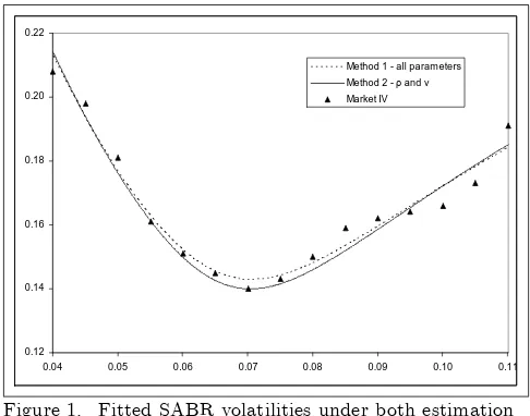
We illustrate the SABR model under both parameterizations by reproducing Figure 3.3 of Haganet al [2]. We use = 0:5 and …t the SABR model using both estimation approaches. This appears in Figure 1 below.
0.12 0.14 0.16 0.18 0.20 0.22
0.04 0.05 0.06 0.07 0.08 0.09 0.10 0.11 Method 1 - all parameters
Method 2 - ρ and ν
Market IV
Figure 1. Fitted SABR volatilities under both estimation methods, = 0:5
The …gure illustrates that the choice of estimation has little e¤ect, and that both methods produce a set of implied volatilities that …t the market volatilities reasonably well. The error sum of squares (SSE) from the …rst method is
SSE1= 2:33 10 4, which is slightly larger than that from the second method,
SSE2= 2:74 10 4. The parameter estimates obtained under both methods
are presented in Table 1. The sets of parameters are very similar.
Table 1. Parameter Estimates
Parameter Method 1 Method 2
0.037561 0.036698
0.5 0.5
0.100044 0.098252
Free Matlab code for parameter estimation under both methods is available atwww.Volopta.com.
4.1
The Backbone
Given values of ; ; andv, we can vary the value off and trace out the ATM volatility B(f; f)from Equation (4) to obtain thebackbone. For a …xed value
of f, if we plot the SABR volatilities B(K; f) from Equation (3), this will
trace out thesmileandskew. This is illustrated in Figure 2, which reproduces Figure 3.1 in Haganet al [2], using the parameters in Table 1 estimated under Method 1 and using a maturityT = 1year.
0.08 0.10 0.12 0.14 0.16 0.18 0.20 0.22
0.04 0.05 0.06 0.07 0.08 0.09 0.10 0.11
Backbone f = 0.065
f = 0.076 f = 0.088
Figure 2. The backbone with its smiles and skews when
= 0
0.08
0.04 0.05 0.06 0.07 0.08 0.09 0.10 0.11
Backbone f = 0.065
f = 0.076 f = 0.088
Figure 3. The backbone with its smiles and skews when
= 1
5
Option Sensitivities
The Greeks from the SABR model resemble those from Black’s model, but contain additional terms to re‡ect the fact that B is not constant. This is
explained by Hagan et al. [2], Lesniewski [3], and Barlett [1].
5.1
Vega
Vega, the sensitivity of the option price to volatility, , is obtained by applying the chain rule on the call price from equation (2) and using equation (3)
Vega= @CB
@ B
@ B
@ (8)
In practice, …nite di¤erences are used to evaluate the derivative @ B
@ , rather
than obtaining this derivative analytically from equation (3).
5.2
Delta
Delta, the sensitivity of the option price to the forward rate, is dependent on the parameterization used. If the …rst parameterization is used then delta is the total derivative
If, on the other hand, the second parameterization is used then delta is
to re‡ect the fact that is a function off:
5.3
Barlett Updated Greeks
Bartlett [1] has proposed re…nements of the Greeks in equations (8) and (9). In this section we explain the development of these updated Greeks.
5.3.1 Updated Delta
The SABR Delta in equation (9) is obtained by assuming a shift in the forward rate while keeping the value of constant
f ! f + f
! :
Bartlett [1] explains that since andf are correlated, a shift inf will likely be accompanied by a shift in . Hence a more realistic scenario is
f ! f + f
! + f :
To calculate f we use the the well-know result that the two correlated
Brownian motionsW1
t andWt2 from equation (1) can be expressed in terms of
twoindependent Brownian motionsWtandZtby setting, for example, dWt1=
dWt and dWt2 = dWt+
p
1 2dZ
t. Hence we can write the SABR model
from equation (1) as
dft = tftdWt (10)
This implies that the volatility process from equation (10) can be written as
d t=
The instantaneous change in volatility,d t, can now be expressed in two terms
(1) the instantaneous change in the forward,dft, and (2) the level of the
volatil-ity, t. The change in volatility due to a change in the forward is the …rst
term
d t
dft
= v
ft :
The SABR delta is updated by including the change in Bbrought on by changes
5.3.2 Updated Vega
Analogously to the SABR Delta, the SABR Vega in equation (8) is updated by assuming a shift in the volatility while keeping the value off constant
f ! f
! + :
Bartlett [1] explains that a more realistic scenario is
f ! f+ f
! + :
Turning to equation (1) again, the forward process can be written
dft = tft dWt+
This implies that the forward process from equation (11) can be written as
dft=
The instantaneous change in volatility, dft, can be expressed in two terms (1)
the instantaneous change in the forward,d t, and (2) the level of the volatility,
t. The change in the forward due to a change in volatility is the …rst term
dft
d t
= ft
v :
The SABR delta is updated by including the change in Bbrought on by changes
in
A free Matlab program for the updated Greeks is available atwww.Volopta.com.
6
SABR Re…nements
The original formula by Hagan et al. [2] in Equation (3) has been shown to break down when the strike is small and the maturity is long. In response, a number of researchers have sought to re…ne the implied volatility. One such re…nement is summarized by Jan Oblój [4], so we state his results here. The implied volatility surface (x; T)for log-moneynessx= log (F=K)and maturity
T can be approximated as
In this expression, we have
IH1 (x) = (1 )
2 2
24 (f K)1 +
v
4 (f K)(1 )=2 +
2 3 2 v2
24 ;
and four cases forI0
B(x).
Case 1: x= 0.
I0(0) = K 1:
Case 2: v= 0:
I0(x) = x (1 )
f1 K1 :
Case 3: = 1:
I0(x) = vx
ln
p
1 2 z+z2+z
1
wherez= vx. Case 4: <1.
I0(x) = vx
ln
p
1 2 z+z2+z
1
wherez= v(f
1
K1 )
(1 ) : As before, the SABR implied volatility B(x; T)
is plugged into Black’s formula in Equation (2), and the price of the call is obtained. A free Matlab program for estimating the SABR parameters under this re…ned scheme is available atwww.Volopta.com.
References
[1] Bartlett, B. (2006). "Hedging Under SABR Model," Wilmott Magazine, July 2006, pp. 2-4.
[2] Hagan, P., Kumar, D., Lesniewski, L, and D.E. Woodward (2002). "Man-aging Smile Risk,"Wilmott Magazine, September 2002, pp. 84-108.
[3] Lesniewski, A. (2008). "The Volatility Cube."
[4] Oblój, J. (2008). "Fine-Tune Your Smile: Correction to Hagan et al," Work-ing Paper, Imperial College, London, UK.