A Learnable Constraint-based Grammar Formalism
Smaranda Muresan
School of Communication and Information Rutgers University
Abstract
Lexicalized Well-Founded Grammar
(LWFG) is a recently developed syntactic-semantic grammar formalism for deep language understanding, which balances expressiveness with provable learnability results. The learnability result for LWFGs assumes that the semantic composition constraints are learnable. In this paper, we show what are the properties and principles the semantic representation and grammar formalism require, in order to be able to learn these constraints from examples, and give a learning algorithm. We also introduce a LWFG parser as a deductive system, used as an inference
engine during LWFG induction. An
example for learning a grammar for noun compounds is given.
1 Introduction
Recently, several machine learning approaches have been proposed for mapping sentences to their formal meaning representations (Ge and Mooney, 2005; Zettlemoyer and Collins, 2005; Muresan, 2008; Wong and Mooney, 2007; Zettlemoyer and Collins, 2009). However, only few of them in-tegrate the semantic representation with a gram-mar formalism: λ-expressions and Combinatory
Categorial Grammars (CCGs) (Steedman, 1996) are used by Zettlemoyer and Collins (2005;2009), and ontology-based representations and Lexical-ized Well-Founded Grammars (LWFGs) (Mure-san and Rambow, 2007) are used by Mure(Mure-san (2008).
An advantage of the LWFG formalism, com-pared to most constraint-based grammar for-malisms developed for deep language understand-ing, is that it is accompanied by a learnability
guarantee, the search space for LWFG induc-tion being a complete grammar lattice (Muresan and Rambow, 2007). Like other constraint-based grammar formalisms, the semantic structures in LWFG are composed by constraint solving, se-mantic composition being realized through con-straints at the grammar rule level. Moreover, se-mantic interpretation is also realized through con-straints at the grammar rule level, providing ac-cess to meaning during parsing.
However, the learnability result given by Mure-san and Rambow (2007) assumed that the gram-mar constraints were learnable. In this paper we present the properties and principles of the seman-tic representation and grammar formalism that al-low us to learn the semantic composition con-straints. These constraints are a simplified version of ”path equations” (Shieber et al., 1983), and we present an algorithm for learning these constraints from examples (Section 5). We also present a LWFG parser as a deductive system (Shieber et al., 1995) (Section 3). The LWFG parser is used as an innate inference engine during LWFG learn-ing, and we present an algorithm for learning LWFGs from examples (Section 4). A discussion and an example of learning a grammar for noun compounds are given is Section 6.
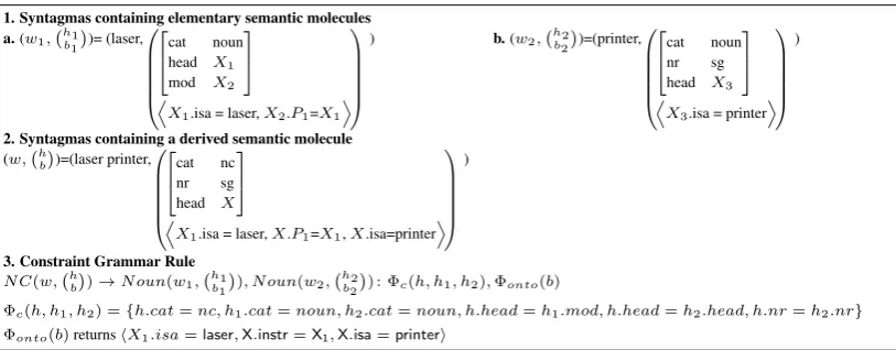
1. Syntagmas containing elementary semantic molecules a.(w1,`h1
b1
´)= (laser,0 B B B B B @ 2 6 4
cat noun head X1
mod X2 3 7 5
D
X1.isa = laser,X2.P1=X1E 1 C C C C C A
) b.(w2,`h2 b2
´)=(printer,0 B B B B B @ 2 6 4
cat noun nr sg head X3
3 7 5
D
X3.isa = printerE 1 C C C C C A
)
2. Syntagmas containing a derived semantic molecule (w,`h
b
´)=(laser printer,0 B B B B B @ 2 6 4
cat nc nr sg head X 3 7 5
D
X1.isa = laser,X.P1=X1,X.isa=printerE 1 C C C C C A
)
3. Constraint Grammar Rule
N C(w,`h b ´
)→N oun(w1,`h1 b1 ´
), N oun(w2,`h2 b2 ´
) : Φc(h, h1, h2),Φonto(b)
Φc(h, h1, h2) ={h.cat=nc, h1.cat=noun, h2.cat=noun, h.head=h1.mod, h.head=h2.head, h.nr=h2.nr}
Φonto(b)returnshX1.isa=laser,X.instr=X1,X.isa=printeri
Figure 1: Syntagmas containing elementary semantic molecules (1) and a derived semantic molecule (2); A constraint grammar rule together with the semantic composition and ontology-based interpreta-tion constraints,ΦcandΦonto(3)
two types of constraints, one for semantic com-position and one for semantic interpretation. The first property allows LWFG learning from a small set of examples. The last two properties make LWFGs a type of syntactic-semantic grammars.
Definition 1. A semantic molecule associated with a natural language stringw, is a syntactic-semantic representation, w0 = hb, where h (head) encodes compositional information, while b (body) is the actual semantic representation of the stringw.
Grammar nonterminals are augmented with pairs of strings and their semantic molecules. These pairs are calledsyntagmas, and are denoted byσ= (w, w0) = (w, hb).
Examples of semantic molecules for the nouns
laser and printer and the noun-noun compound
laser printer are given in Figure 1. When as-sociated with lexical items, semantic molecules are calledelementary semantic molecules. When semantic molecules are built by the combina-tion of others, they are called derived semantic molecules. Formally, the semantic molecule head,
h, is a one-level feature structure (i.e., values are
atomic), while the semantic molecule body,b, is a
logical form built as a conjunction of atomic pred-icateshconcepti.hattri=hconcepti, where vari-ables are either concept or slot identifiers in an on-tology.1
1The body of a semantic molecule is called OntoSeR and
Muresan and Rambow (2007) formally defined LWFGs, and we present here a slight modification of their definition.
Definition 2. A Lexicalized Well-Founded Gram-mar (LWFG) is a 7-tuple, G = hΣ,Σ0, NG, , PG, PΣ, Si, where:
1. Σis a finite set of terminal symbols.
2. Σ0 is a finite set of elementary
seman-tic molecules corresponding to the terminal symbols.
3. NG is a finite set of nonterminal symbols. NG∩Σ =∅. We denotepre(NG)⊆NG, the set of pre-terminals (a.k.a, parts of speech) 4. is a partial ordering relation among
non-terminals.
5. PGis the set of constraint grammar rules. A constraint grammar rule is written A(σ) →
B1(σ1), . . . , Bn(σn) : Φ(¯σ), whereA, Bi ∈ NG, σ¯ = (σ, σ1, ..., σn) such that σ =
(w, w0), σi = (wi, wi0),1 ≤ i ≤ n, w = w1· · ·wn, w0 = w01◦ · · · ◦wn0, and◦is the composition operator for semantic molecules (more details about the composition oper-ator are given in Section 5). For brevity,
we denote a rule by A → β: Φ, where
A ∈ NG, β ∈ NG+. PΣ is the set of con-straint grammar rules whose left-hand side are pre-terminals, A(σ) →,A ∈ pre(NG).
We use the notation A → σ for this gram-mar rules. In LWFG due to partial ordering among nonterminals we can have ordered constraint grammar rules and non-ordered constraint grammar rules (both types can be recursive or non-recursive). A grammar rule A(σ) → B1(σ1), . . . , Bn(σn) : Φ(¯σ), is an ordered rule, if for allBi, we haveA Bi. In LWFGs, each nonterminal symbol is a left-hand side in at least one ordered non-recursive rule and the empty string cannot be derived from any nonterminal symbol. 6. S∈NGis the start nonterminal symbol, and
∀A∈NG, S A(we use the same notation for the reflexive, transitive closure of).
The partial ordering relationmakes the set of nonterminals well-founded2, which allows the
or-dering of the grammar rules, as well as the order-ing of the syntagmas generated by LWFGs. This ordering allow LWFG learning from a small set of representative examples (Muresan and Rambow, 2007) (PΣis not learned).
An example of a LWFG rule is given in Fig-ure 1(3). Nonterminals are augmented with syn-tagmas. Moreover, in LWFG the semantic com-position and interpretation are realized via con-straints at the grammar rule level (Φ(¯σ) in Defi-nition 2). More precisely, syntagma composition means string concatenation (w = w1w2) and
se-mantic molecule composition ( h b
= h1b1◦ h2b2) —- where the bodies of semantic molecules are concatenated through logical conjunction (b = (b1, b2)ν, where ν is a variable substitutionν = {X2/X, X3/X}), while the semantic molecules
heads are composed through compositional con-straintsΦc(h, h1, h2), which are a simplified
ver-sion of “path equations” (Shieber et al., 1983) (see Figure 1(3)). During LWFG learning, composi-tional constraintsΦcare learnedtogether with the
grammar rules. Semantic interpretation, which is ontology-based in LWFG, is also encoded as constraints at the grammar rule level — Φonto
— providing access to meaning during parsing. Φonto(b) constraints are applied to the body of
the semantic molecule corresponding to the
syn-2should not be confused with information ordering
de-rived from flat feature structures
tagma associated with the left-hand side nonter-minal. The ontology-based constraints are not learned; rather, Φontois a general predicate that
succeed or fail as a result of querying an ontology — when it succeeds, it instantiates the variables of the semantic representation with concepts/slots in the ontology (see the example in Figure 1(3)).
2.1 Derivation in LWFG
The derivation in LWFG is called ground syn-tagma derivation, and it can be seen as the bottom up counterpart of the usual derivation. Given a LWFG,G, theground syntagma deriva-tion relation, ∗⇒G, is defined as: A→σ
A∗G⇒σ (if σ =
(w, w0), w ∈ Σ, w0 ∈ Σ0, i.e., A ∈ pre(NG, ),
andBi∗⇒Gσi, i=1,...,n, A(σ)→B1(σ1),...,Bn(σn) : Φ(¯σ)
A∗⇒Gσ .
Theset of all syntagmasgenerated bya gram-mar G is Lσ(G) = {σ|σ = (w, w0), w ∈
Σ+,∃A ∈ NG, A ∗⇒G σ}. Given a LWFG G, Eσ ⊆ Lσ(G) is called a sublanguage ofG.
Ex-tending the notation, given a LWFGG, the set of
syntagmas generated by arule(A→β: Φ)∈PG
is Lσ(A → β: Φ) = {σ|σ = (w, w0), w ∈
Σ+,(A → β: Φ) ∗⇒G σ}, where(A → β: Φ) ∗⇒G
σdenotes the ground derivationA ∗⇒Gσ obtained
using the rule A → β: Φin the last derivation step.
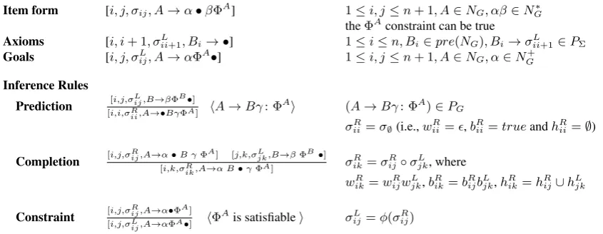
3 LWFG Parsing as Deduction
Following Shieber (1995), we present the Lexical-ized Well-Founded Grammar parser as a deduc-tive proof system in Table 1. The items of the logic are of the form [i, j, σij, A → α •βΦA],
whereA → αβ: ΦA is a grammar rule, ΦA — the constraints corresponding to the grammar rule whose left-hand side nonterminal isA— can be
true, • shows how much of the right-hand side of the rule has been recognized so far,ipoints to
the parent node where the rule was invoked, andj
points to the position in the input that the recogni-tion has reached. We use the following notarecogni-tions:
σR
ij = (wijR, hR
ij
bR ij
) are syntagmas corresponding to the partially parsed right-hand side of a rule;
σijL = (wLij, hLij
bL ij
non-Item form [i, j, σij, A→α•βΦA] 1≤i, j≤n+ 1, A∈NG, αβ∈NG∗
theΦAconstraint can be true
Axioms [i, i+ 1, σL
ii+1, Bi→ •] 1≤i≤n, Bi∈pre(NG), Bi→σiiL+1∈PΣ
Goals [i, j, σL
ij, A→αΦA•] 1≤i, j≤n+ 1, A∈NG, α∈NG+
Inference Rules
Prediction [i,j,σLij,B→βΦB•]
[i,i,σR
ii,A→•BγΦA] h
A→Bγ: ΦA
i (A→Bγ: ΦA)
∈PG
σR
ii =σ∅(i.e.,wiiR=,bRii=trueandhRii=∅)
Completion [i,j,σijR,A→α•B γΦA] [j,k,σjkL,B→βΦB•]
[i,k,σR
ik,A→α B•γΦA]
σikR =σijR◦σjkL, where
wR
ik=wijRwLjk,bRik=bijRbLjk,hRik=hRij∪hLjk
Constraint [i,j,σijR,A→α•ΦA]
[i,j,σL
ij,A→αΦA•] h
ΦAis satisfiable
i σL
ij=φ(σRij)
Table 1: LWFG parsing as deductive system
terminal of a LWFG rule). The goal items are of the form [i, j, σijL, A → αΦA•], where σLij is
ground-derived from the ruleA→α: ΦA.
Compared to the deductive system in (Shieber et al., 1995), the LWFG parser has the follow-ing characteristics: each item is augmented with a syntagma; the Constraint rule is a new infer-ence rule, and the goal items are associated to
every nonterminal in the grammar, not only to the start symbol (i.e., LWFG parser is a robust parser). TheConstraintinference rule is the only one that obtains an inactive edge3, from an active
edge by executing the grammar constraintΦA(the
•is shifted across the constraint). By applying the
Constraint rule as the last inference rule we obtain the ground-derived syntagmasσijL. Thus, the goal
items are obtained only after the Constraint rule is applied. During this inference rule we have that
σijL = φ(σijR), whereφis defined by: wijL = wijR, bL
ij = bRijνij, andhLij = ϕ(hRij). The substitution νij and the functionϕare implicitly contained in
the grammar constraintΦAc(hLij, hRij)(see Section 5 for details)
Definition 3(Robust parsing provability). Robust parsing provability corresponds to reaching the goal item:`rp A(σLij)iff[i, j, σijL, A→αΦA•].
Thus, we can notice that the ground syntagma derivation is equivalent to robust parsing provabil-ity, i.e.,A∗⇒GσiffG`rp A(σ).
3We use Kay’s terminology: items are edges, where the
axioms and goals are inactive edges having• at the end, while the rest are active edges (Kay, 1986).
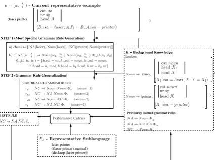
4 Learning LWFGs
The theoretical learning model for LWFG induc-tion, Grammar Approximation by Representative Sublanguage (GARS), together with a learnability theorem was introduced in (Muresan and Ram-bow, 2007). LWFG’s learning framework char-acterizes the “importance” of substructures in the model not simply by frequency, but rather lin-guistically, by defining a notion of “representa-tive examples” that drives the acquisition process. Informally, representative examples are “building blocks” from which larger structures can be in-ferred via reference to a larger generalization cor-pus referred to as representative sublanguage in (Muresan and Rambow, 2007). The GARS model uses a polynomial algorithm for LWFG learning that take advantage of the building blocks nature of representative examples.
The LWFG induction algorithm belongs to the class of Inductive Logic Programming methods (ILP), based on entailment (Muggleton, 1995; Dzeroski, 2007). At each step a new constraint grammar rule is learned from the current repre-sentative example, σ. Then this rule is added to the grammar rule set. The process continues until all the representative examples are covered. We describe below the process of learning a grammar rule from the current representative example:
STEP 1 (Most Specific Grammar Rule Generation)
STEP 2 (Grammar Rule Generalization) (laser printer,
CANDIDATE GRAMMAR RULES
laser printer Performance Criteria
BEST RULE
((laser printer) manual) (desktop (laser printer))
K ! Background Knowledge
Lexicon
(laser, )
Previously learned grammar rules
cat nc
)
(printer, )
σ= (w,!h b
"
)- Current representative example
a) chunks={[NA(laser), Noun(laser)], [NC(printer),Noun(printer)]}
rg1 NC→Noun Noun: Φc4 (score=1)
rg2 NC→NA Noun: Φc5 (score=2)
b) r:NC(w,!h b
"
)→Noun(w1,!h1
b1 "
)Noun(w2,!h2
b2 "
): Φc4(h, h1, h2) Φc4(h, h1, h2) ={h.cat=nc, h1.cat=noun, h2.cat=noun,
Eσ- Representative Sublanguage
NC→NA NC: Φc7
rg4 NC→NA NC: Φc7 (score=3)
rg3 NC→Noun NC: Φc6 (score=2)
Noun→
catnoun
headX1
modX2
"X1.isa=laser, X2.Y=X1#
catnoun
"X3.isa=printer# NA→Noun: Φc1
"B.isa=laser, A.P1=B, A.isa=printer#
NA→NA NA: Φc2
NC→Noun: Φc3
nr sg
headA
headX3
nr sg Noun→ h.head=h1.mod, h.head=h2.head, h.nr=h2.nr}
Figure 2: Example of Grammar Rule Learning
in the representative example gives the left-hand-side nonterminal, while a robust parser returns the minimum number of chunks covering the representative example. The categories of the chunks give the non-terminals of the right-hand side of the most specific rule. For example, in Figure 2, given the representative example laser printer
annotated with its semantic molecule, and the background knowledge containing the already learned rules N A → N oun: Φc1, N A → N A N A: Φc2,N C → N oun: Φc3
the robust parser generates the chunks corresponding to the noun laser and the noun printer: [NA(laser),Noun(laser)] and [NC(printer),Noun(printer)], re-spectively. The most specific rule is
N C → N oun N oun: Φc4, where the
left-hand side nonterminal is given by the category of the representative example, in this casenc. Compositional constraintsΦc4
are learned as well. In section 5 we give the algorithm for learning these constraints, and several properties and principles that are needed in order for these constraints to be learnable.
2. Grammar Rule Generalization. In the sec-ond step, this most specific rule is gener-alized, obtaining a set of candidate gram-mar rules (the generalization step is the in-verse of the derivation step used to define the complete grammar lattice search space in
(Muresan and Rambow, 2007)). The perfor-mance criterion in choosing the best gram-mar rule among these candidate hypotheses is the number of examples in the representa-tive sublanguage Eσ (generalization corpus)
that can be parsed using the candidate gram-mar rule, rgi in the last ground derivation
step, together with the previous learned rules, i.e.,|Eσ∩Lσ(rgi)|. In Figure 2 given the
rep-resentative sublanguageEσ={ laser printer, laser printer manual, desktop laser printer}
the learner will generalize to the recursive rule N C → N A N C: Φ7, since only this
rule can parse all the examples inEσ.
5 Learnable Composition Constraints In LWFG, the semantic structures are composed by constraint solving, rather than functional ap-plication (with lambda expressions and lambda re-duction). This section presents the properties and principles that guarantee the learnability of the compositional constraints,Φc, and presents an
al-gorithm to generate these constraints from exam-ples, which is a key result for LWFG learnability. The information for semantic composition is encoded in the head of semantic molecules. There are three types of attributes that belong to the se-mantic molecule headh: category attributes Ac
h,
variable attributesAv
h, and feature attributes A f h.
Thus,Ah = Ach∪ Avh ∪ A f
h andAch,Avh,A f h are
pairwise disjoint. For example, in Figure 1 for the noun-noun compoundlaser printer, we have that
Ac
h = {cat}, A f
h = {nr}, and Avh = {head},
while for the noun laser we have that Ac
h1 =
{cat},Afh1 =∅, andAv
h1 ={head, mod}(nouns
can be modifiers of other nouns, so their represen-tation is similar to that of an adjective).
We describe in turn each of these types of at-tributes and their corresponding principles. All principles, except the first and the last mirror principles in other constraint-based linguistic for-malisms, such as HPSG (Pollard and Sag, 1994).
The category attributes Ach are state
at-tributes, and their value set gives the category of the semantic molecule. There is one attribute,cat ∈ Ach, which is mandatory and whose value is the
1). The category of a semantic molecule can be given by: 1) thecatattribute alone, or 2) thecat
attribute together with other state attributes inAc h
which are syntactic-semantic markers.
Principle 1(Category Name Principle). The cat-egory nameh.catof a syntagmaσ = (w, hb)is
the same as the grammar nonterminal augmented with syntagmaσ.
When learning a LWFG rule from an example
σ, the above principle allows us to determine the
nonterminal in the left-hand side of the grammar rule. For example, when learning the LWFG rule from the syntagma corresponding tolaser printer
in Figure 2, the nonterminal in the left-hand side of the LWFG rule isN Csinceh.cat=nc.
The variable attributes Av
h are attributes
whose values are logical variables and represent the semantic valence of the molecule, which al-lows the binding of the semantic representations. These logical variables appear in the semantic molecule body as well. For example, in Figure 1(2) for the noun-noun compound laser printer, the value of the variable attributehead ∈ Av
h is
a variable X, which appears also in the body of
the semantic moleculehX1.isa=laser, X.P1 = X1, X.isa=printeri. It can be noticed that the
semantic molecule body contains other variables as well (X1, P1). However, only the variables
present in the semantic molecule head as well (X)
will participate in further composition.
Principle 2 (Semantic Representation Binding Principle). All the logical variables that the body bof a semantic molecule corresponding to a syn-tagmaσ = (w, hb), share with other syntagmas,
are at the same time values of the variable at-tributes (Avh) of the semantic molecule head.
There is one variable attribute,head∈ Av hthat
represents the head of a syntagma, giving the fol-lowing principle:
Principle 3 (Semantic Head Principle). Given a syntagma σ = (w, hb) ground derived from a
grammar rule, r, there exists one and only one syntagmaσi = (wi, hbii)corresponding to a non-terminal Bi in rule r’s right-hand side, which has the same value of the attribute head, i.e., h.head=hi.head.
The feature attributes Afh are the attributes
whose values express the specific properties of the semantic molecules (e.g., number, person).
Principle 4 (Feature Inheritance Principle). If σi = (wi, hbii
)is the semantic head of a
ground-derived syntagma σ = (w, hb), then all
fea-ture attributes ofσ inherit the values of the cor-responding attributes that belong to the seman-tic headσi. That is, ifh.head = hi.head, then h.f =hi.f,∀f ∈ Afh∩Afhi.
Besides this principle, the feature attributes are used for category agreement. The categories that enter in agreement are maximum projection cat-egories. This linguistic knowledge about agree-ment is used in the form of the following princi-ple:
Principle 5 (Feature Agreement Principle). The agreeing categories and the agreement features are a-priori given based on linguistic knowledge, and are applied only at the semantic head level.
Given all the above principles, we can now for-mulate the general Composition Principle:
Principle 6(Composition Principle). A syntagma σ = (w, w0) corresponding to the left-hand side
nonterminal of a grammar rule is obtained by string concatenation (w = w1. . . wn) and the composition of semantic molecules corresponding to the nonterminals from the rule right-hand side:
w0=
h b
= (w1· · ·wn)0 =w01◦ · · · ◦w0n
=
h1 b1
◦ · · · ◦
hn bn
=
h1◦ · · · ◦hn hb1, . . . , bniν
The composition of the semantic molecule bod-ies is realized through conjunction after the ap-plication of a variable substitution ν. The body
variable specialization substitution ν is the most general unifier (mgu) of b and b1, . . . , bn, s.t b = (b1, . . . , bn)ν. It is a particular form of the
commonly used substitution (Lloyd, 2003), i.e., a finite set of the form {X1/Y1, . . . , Xm/Ym},
whereX1, . . . , Xm, Y1, . . . , Ymare variables, and X1, . . . , Xmare distinct.
similar to “path equations” (Shieber et al., 1983; van Noord, 1993), but applied to flat feature struc-tures:
hi.c=ct
hi.vi=hj.vj
hi.f=ct or
hi.f=hj.f where
0≤i, j≤n, i6=j c∈ Achi
vi∈ Avhi, vj∈ A
v hj
f∈ Afhi, f∈ Afhj
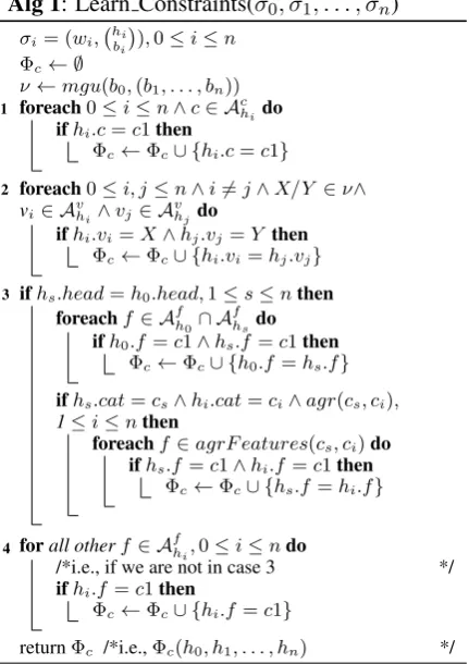
When learning a LWFG rule from a repre-sentative example σ as in Figure 2, the robust
parser returns the minimum number of chunks,
n, covering σ. The body variable substitutionν
is fully determined by the representative exam-ple as mgu of b andb1, . . . , bn, and the
compo-sitional constraintsΦc(h, h1, . . . , hn)are learned
using Alg 1. For example, in Figure 2, when learning from the representative example corre-sponding to the stringlaser printer, we have that
ν ={X1/B, X2/A, X3/A, Y /P1}.
In Alg 1 we use the notationσ0= (w0, h0b0)to
denote the representative exampleσ.
Alg 1: Learn Constraints(σ0, σ1, . . . , σn)
σi= (wi,
`hi
bi
´
),0≤i≤n
Φc← ∅
ν←mgu(b0,(b1, . . . , bn))
foreach0≤i≤n∧c∈ Ac hido
1
ifhi.c=c1then
Φc←Φc∪ {hi.c=c1}
foreach0≤i, j≤n∧i6=j∧X/Y ∈ν∧ 2
vi∈ Avhi∧vj∈ A
v hjdo
ifhi.vi=X∧hj.vj=Y then Φc←Φc∪ {hi.vi=hj.vj}
ifhs.head=h0.head,1≤s≤nthen
3
foreachf∈ Afh0∩ Afhsdo
ifh0.f=c1∧hs.f=c1then Φc←Φc∪ {h0.f=hs.f}
ifhs.cat=cs∧hi.cat=ci∧agr(cs, ci),
1≤i≤nthen
foreachf∈agrF eatures(cs, ci)do
ifhs.f=c1∧hi.f=c1then Φc←Φc∪ {hs.f=hi.f}
forall otherf∈ Afhi,0≤i≤ndo
4
/*i.e., if we are not in case 3 */ ifhi.f=c1then
Φc←Φc∪ {hi.f=c1}
returnΦc /*i.e.,Φc(h0, h1, . . . , hn) */
In the first step, the constraints corresponding to category attributes are fully determined by the
values of these attributes that appear in the se-mantic molecule heads of σ0, . . . σn. In Figure
2, when learning the most specific rule r from the representative example laser printer, the set of constraints{h.cat=nc, h1.cat=noun, h2= noun} ⊂ Φc4 are the constraints corresponding
to category attributes. In the second step, the con-straints corresponding to variable attributes are fully determined by the variables in the substitu-tion ν that also appear as values of variable
at-tributes hi.vi, hj.vj, where 0 ≤ i, j ≤ n and i 6= j. In Figure 2, only {X2/A, X3/A} ⊂ ν
will be used, generating the set of constraints
{h.head=h1.mod, h.head=h2.head} ⊂ Φc4.
In the third step, the values of the feature at-tributes which obey Principles 4 and 5 are gen-eralized — agr(cs, ci) is the predicate which gives
us the agreement between the categories cs and ci (e.g., the subject agrees with the verb), and
agrFeatures(cs, ci) gives us the set of feature
at-tributes that participate in agreement (e.g., nr, pers, case). In Figure 2, the set of constraints
{h.nr = h2.nr} ⊂ Φc4 represents the
general-ization of the feature attribute values fornr, using
Principle 4 . For all features attributes besides the ones that obey the above two principles, the gener-ated constraints keep the particular values of these attributes (step 4 of Alg 1).
6 Examples
gener-A. Learning Examples:
) 5. (laser printer manual,0 B
2. (laser printer,0 B
) 6. (desktop laser printer,0 B
3. (printer,0 B
A.isa = printerE 1
) 7. (laser printer manual,0 B
4. (laser printer,0 B
B.isa = laser, A.P1=B, A.isa=printer
E
) 8. (desktop laser printer,0 B
B.isa = desktop, A.P1=B, C.isa=laser, A.P2=C, A.isa=printer
E
B. Learned LWFG Rules:
NA(w,“hb”)→Noun(w1,
Figure 3: Learning LWFG Rules for Noun-Noun Compounds
alization (5-8). The learned grammar rules, in-cluding the learned composition constraints are also shown. The first two LWFG rules ground de-rive syntagmas for noun adjuncts, while the last two rules ground derive syntagmas for noun com-pounds. For example, ”desktop laser printer” can be either a fully-formed noun compound (cate-gory nc), or it can be further combined with the noun ”invoice” to obtain ”desktop laser printer in-voice”, case in which it is a noun adjunct (cate-gory na). The learned rule for noun adjuncts is
both left and right recursive, accounting for both left and right-branching noun compounds. Even though we can obtain overgeneralization in syn-tax, the ontology-based interpretation constraint at the rule level will prune some erroneous parses. Preliminary results in the medical domain show thatΦontocan help remove erroneous parses even
when using just a weak ontological model (se-mantic roles of verbs, prepositions, attributes of adjectives and adverbs, but no synonymy, or
hi-erarchy of concepts or roles). However, more ex-periments need to be run for reporting quantitative results.
7 Conclusions
We have presented the properties and princi-ples that the semantic representation integrated in LWFG requires so that the semantic compo-sitional constraints are learnable from examples. These properties together with Alg 1 give a the-oretical result that in conjunction with the learn-ability result of Muresan and Rambow (2007) show that LWFG is a learnable constraint-based grammar formalism that can be used for deep lan-guage understanding. Instead of writing grammar rules and constraints by hand, one needs to pro-vide only a small set of annotated examples.4
4The author acknowledges the support of the NSF (SGER
References
Dzeroski, Saso. 2007. Inductive logic programming in a nutshell. In Getoor, Lise and Ben Taskar, editors,
Introduction to Statistical Relational Learning. The
MIT Press.
Ge, Ruifang and Raymond J. Mooney. 2005. A statis-tical semantic parser that integrates syntax and
se-mantics. InProceedings of CoNLL-2005.
Kay, M. 1986. Algorithm schemata and data struc-tures in syntactic processing. InReadings in natural
language processing, pages 35–70. Morgan
Kauf-mann Publishers Inc., San Francisco, CA, USA.
Lloyd, John W. 2003. Logic for Learning:
Learn-ing Comprehensible Theories from Structured Data.
Springer, Cognitive Technologies Series.
Muggleton, Stephen. 1995. Inverse Entailment and
Progol. New Generation Computing, Special Issue
on Inductive Logic Programming, 13(3-4):245–286.
Muresan, Smaranda and Owen Rambow. 2007. Gram-mar approximation by representative sublanguage:
A new model for language learning. InProceedings
of the 45th Annual Meeting of the Association for
Computational Linguistics (ACL).
Muresan, Smaranda. 2008. Learning to map text to graph-based meaning representations via
gram-mar induction. In Coling 2008: Proceedings of
the 3rd Textgraphs workshop on Graph-based
Al-gorithms for Natural Language Processing, pages
9–16, Manchester, UK, August. Coling 2008 Orga-nizing Committee.
Neumann, G¨unter and Gertjan van Noord. 1994. Re-versibility and self-monitoring in natural language
generation. In Strzalkowski, Tomek, editor,
Re-versible Grammar in Natural Language Processing,
pages 59–96. Kluwer Academic Publishers, Boston.
Pollard, Carl and Ivan Sag. 1994. Head-Driven
Phrase Structure Grammar. University of Chicago
Press, Chicago, Illinois.
Shieber, Stuart, Hans Uszkoreit, Fernando Pereira, Jane Robinson, and Mabry Tyson. 1983. The
formalism and implementation of PATR-II. In
Grosz, Barbara J. and Mark Stickel, editors,
Re-search on Interactive Acquisition and Use of
Knowl-edge, pages 39–79. SRI International, Menlo Park,
CA, November.
Shieber, Stuart, Yves Schabes, and Fernando Pereira. 1995. Principles and implementation of deductive
parsing. Journal of Logic Programming, 24(1-2):3–
36.
Steedman, Mark. 1996. Surface Structure and
Inter-pretation. The MIT Press.
van Noord, Gertjan. 1993. Reversibility in Natural
Language Processing. Ph.D. thesis, University of
Utrecht.
Wong, Yuk Wah and Raymond Mooney. 2007. Learn-ing synchronous grammars for semantic parsLearn-ing
with lambda calculus. InProceedings of the 45th
Annual Meeting of the Association for
Computa-tional Linguistics (ACL-2007).
Zettlemoyer, Luke S. and Michael Collins. 2005. Learning to map sentences to logical form: Struc-tured classification with probabilistic categorial
grammars. InProceedings of UAI-05.
Zettlemoyer, Luke and Michael Collins. 2009. Learn-ing context-dependent mappLearn-ings from sentences to logical form. InProceedings of the Association for