Thesis by
Zhenhua Liu
In Partial Fulfillment of the Requirements for the Degree of
Doctor of Philosophy
California Institute of Technology Pasadena, California
2014
c
2014
This thesis is dedicated to
my wife Zheng,
whose love made this possible,
my parents,
who have supported me all the way,
Acknowledgments
During the past five years, I have been always grateful for the extreme fortune to be co-advised by Prof. Adam Wierman and Prof. Steven Low. It is really a luxury and indeed an honor, working with them at this early stage of my academic career, and learning from them from critical thinking, clear writing, effective presentations, student mentoring, time management, positive attitude, and many others. The experience has far surpassed my expectation. Their thoughtful guidance, continuing support without reservation, and cheerful encouragement accompanied me to hurdle all the obstacles during the past years. They did motivate and nurture me so much that I feel even stronger than I ever imagined. In my mind, they are the best advisors and excellent role models! It feels like such a short five years and I still have quite a lot to learn, but it is already the time to move on. They are my most important motivation in pursuing an academic position because I sincerely appreciate all the amazing impacts they have had on me, and hope to extend these to others through my own career in the future.
I am also grateful to many other collaborators all over the world. First, the past three-year collaborations with HP Labs contribute a lot to my knowledge and skills. My mentor, Yuan Chen, has always been patient and ready to help. We did an excellent job together with great colleagues, including Cullen Bash, Chandrakant Patel, Daniel Gmach, Zhikui Wang, Manish Marwah, Chris Hyser, and many others. This has been a pleasant and productive experience. Second, I would like to thank those from Caltech: Minghong Lin, Niangjun Chen, Benjamin Razon, Iris Liu, and Katie Knister. It has been a great pleasure working with them. In particular, I would like to thank Prof. Mani Chandy for his insightful comments and advice. I am also thankful to my former advisors, Prof. Youjian Zhao and Prof. Xiaoping Zhang, for their guidance during my master study in Tsinghua University. Last but not least, I would like to take this opportunity to express my gratitude to many others who helped me during my PhD study: Prof. Xue Liu from McGill University, Prof. Martin Arlitt from University of Calgary and HP Labs, Prof. Jean Walrand from UC Berkeley, Prof. Lachlan Andrew from Australia, Pablo Bauleo from Fort Collins Utilities, Yanpei Chen from Cloudera, and Hao Wang from Google. They all contributed to this thesis from different perspectives and significantly improved its quality.
Caltech, in which students rarely have to worry about anything other than our research. My in-terdisciplinary research benefits quite a bit from Caltech’s open and friendly atmosphere. There is hardly any barrier among different departments or colleges. I believe this contributes a lot to our success and actually I have been actively looking for similar environment during my academic job hunting. Additionally, I would like to thank the helpful administrative staff in our department, especially Maria Lopez and Sydney Garstang, for keeping everything working in our favor.
Abstract
Energy and sustainability have become one of the most critical issues of our generation. While the abundant potential of renewable energy such as solar and wind provides a real opportunity for sustainability, their intermittency and uncertainty present a daunting operating challenge. This thesis aims to develop analytical models, deployable algorithms, and real systems to enable efficient integration of renewable energy into complex distributed systems with limited information.
The first thrust of the thesis is to make IT systems more sustainable by facilitating the integration of renewable energy into these systems. IT represents the fastest growing sectors in energy usage and greenhouse gas pollution. Over the last decade there are dramatic improvements in the energy efficiency of IT systems, but the efficiency improvements do not necessarily lead to reduction in energy consumption because more servers are demanded. Further, little effort has been put in making IT more sustainable, and most of the improvements are from improved “engineering” rather than improved “algorithms”. In contrast, my work focuses on developing algorithms with rigorous theoretical analysis that improve the sustainability of IT. In particular, this thesis seeks to exploit the flexibilities of cloud workloads both (i) in time by scheduling delay-tolerant workloads and (ii) in space by routing requests to geographically diverse data centers. These opportunities allow data centers to adaptively respond to renewable availability, varying cooling efficiency, and fluctuating energy prices, while still meeting performance requirements. The design of the enabling algorithms is however very challenging because of limited information, non-smooth objective functions and the need for distributed control. Novel distributed algorithms are developed with theoretically provable guarantees to enable the “follow the renewables” routing. Moving from theory to practice, I helped HP design and implement industry’s first Net-zero Energy Data Center.
Contents
Acknowledgments iv
Abstract vi
1 Introduction 1
2 Sustainable IT: Greening Geographical Load Balancing 5
2.1 Model and Notation . . . 7
2.1.1 The workload model . . . 7
2.1.2 The data center cost model . . . 7
2.1.3 The geographical load balancing problem . . . 9
2.1.4 Practical considerations . . . 11
2.2 Characterizing the optima . . . 11
2.3 Algorithms . . . 12
2.4 Case study . . . 18
2.4.1 Experimental setup . . . 19
2.4.2 Performance evaluation . . . 21
2.5 Social impact . . . 24
2.5.1 Experimental setup . . . 24
2.5.2 The importance of dynamic pricing . . . 25
2.6 Summary . . . 27
3 Sustainable IT: System Design and Implementation 28 3.1 Sustainable Data Center Overview . . . 30
3.1.1 Power Infrastructure . . . 31
3.1.2 Cooling Supply . . . 32
3.1.3 IT Workload . . . 33
3.2 Modeling and Optimization . . . 34
3.2.2 System Model . . . 37
3.2.3 Cost and Revenue Model . . . 38
3.2.4 Optimization Problem . . . 39
3.2.5 Properties of the optimal workload management . . . 40
3.3 System Prototype . . . 42
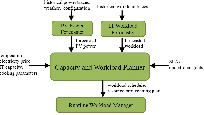
3.3.1 Capacity and Workload Planner . . . 43
3.3.2 PV Power Forecaster . . . 45
3.3.3 IT Workload Forecaster . . . 46
3.3.4 Runtime Workload Manager . . . 47
3.4 Evaluation . . . 47
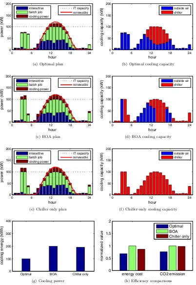
3.4.1 Case Studies . . . 47
3.4.2 Impacts of prediction errors and workload characteristics . . . 54
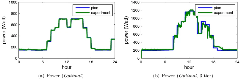
3.4.3 Experimental Results on a Testbed . . . 56
3.5 Summary . . . 58
4 IT for Sustainability: Data Center Demand Response 59 4.1 Coincident peak pricing . . . 62
4.1.1 An overview of coincident peak pricing . . . 62
4.1.2 A case study: Fort Collins Utilities Coincident Peak Pricing (CPP) Program 63 4.2 Modeling . . . 66
4.2.1 Power Supply Model . . . 67
4.2.2 Power Demand Model . . . 68
4.2.3 Total data center costs . . . 70
4.3 Algorithms . . . 70
4.3.1 Expected cost optimization . . . 72
4.3.2 Robust optimization . . . 74
4.3.3 Implementation considerations . . . 76
4.4 Case study . . . 77
4.4.1 Experimental setup . . . 78
4.4.2 Experimental results . . . 80
4.5 Summary . . . 82
5 IT for Sustainability: Pricing Data Center Demand Response 84 5.1 Quantifying the potential of data center demand response . . . 88
5.1.1 Setup . . . 88
5.1.2 Case studies . . . 92
5.3 Prediction-based pricing for data center demand response . . . 98
5.3.1 Model formulation . . . 99
5.3.2 The efficiency of prediction-based pricing . . . 100
5.3.3 Prediction-based pricing versus supply function bidding . . . 104
5.4 Incorporating network constraints . . . 105
5.4.1 Modeling the network . . . 105
5.4.2 Prediction-based pricing in networks . . . 106
5.4.3 The efficiency of prediction-based pricing in networks . . . 108
5.5 Summary . . . 110
6 Concluding remarks 111 6.1 Opportunities for data center participation in demand response programs . . . 112
6.1.1 Opportunities for passive participation . . . 112
6.1.2 Opportunities for active participation . . . 114
6.2 Challenges that limit data center participation in demand response . . . 117
6.3 Recent progress in data center demand response . . . 118
6.3.1 Managing data center participation in demand response . . . 119
6.3.2 Design of market programs appropriate for data centers . . . 120
6.4 Future directions . . . 121
Bibliography 123 Appendices 139 A Appendix: Proofs for Chapter 2 139 A.1 Optimality conditions . . . 139
A.2 Characterizing the optima . . . 141
A.3 Proofs for Algorithm 1 . . . 143
A.4 Proofs for Algorithm 2 . . . 144
A.5 Proofs for Algorithm 3 . . . 147
B Appendix: Proofs for Chapter 3 150 B.1 Proof of Theorem 8 . . . 150
B.2 Proof of Theorem 9 . . . 150
B.3 Proof of Theorem 10 . . . 151
B.4 Proof of Theorem 11 . . . 152
D Appendix: Proofs of Chapter 5 160
D.1 Proof of Theorem 14 . . . 160
D.2 Proof of Theorem 15 . . . 161
D.3 Proof of Theorem 16 . . . 162
D.4 Proof of Corollary 1 . . . 163
List of Figures
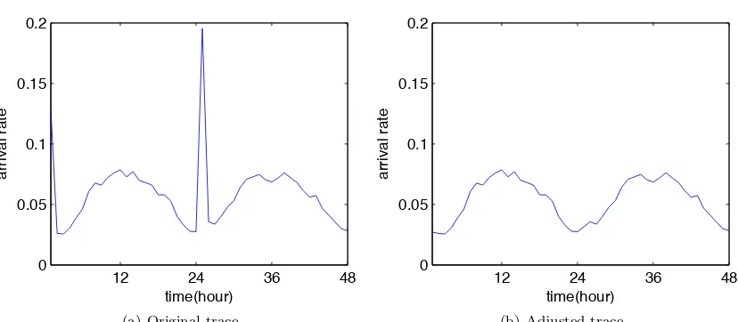
2.1 Hotmail trace used in numerical results. . . 19
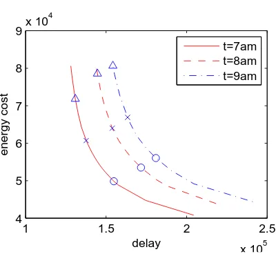
2.2 Pareto frontier of the GLB-Q formulation as a function ofβ for three different times (and thus arrival rates), PDT. Circles, x-marks, and triangles correspond to β = 0.4, 1, and 2.5, respectively. . . 20
2.3 Convergence of all three algorithms. . . 21
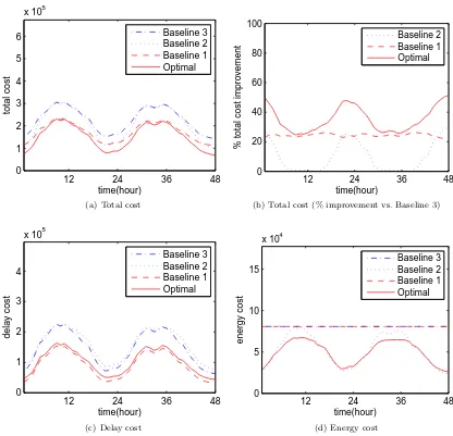
2.4 Impact of ignoring network delay and/or energy price on the cost incurred by geo-graphical load balancing. . . 23
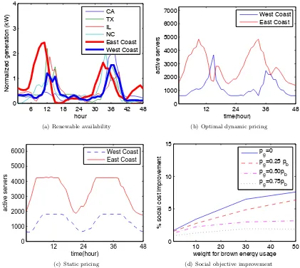
2.5 Geographical load balancing “following the renewables”. (a) Renewable availability. (b) and (c): Capacity provisionings of east coast and west coast data centers when there are renewables, under (b) optimal dynamic pricing and (c) static pricing. (d) Reduction in social cost from dynamic pricing compared to static pricing as a function of the weight for brown energy usage, 1/β˜, and ˜β = 0.1. . . 26
3.1 Sustainable Data Center . . . 30
3.2 One week renewable generation . . . 31
3.3 One week real-time electricity price . . . 32
3.4 One week interactive workload . . . 33
3.5 Cooling coefficient comparison, for conversion, 20◦C=68◦F, 25◦C=77◦F, 30◦C=86◦F . 35 3.6 Optimal cooling power . . . 36
3.7 System Architecture . . . 43
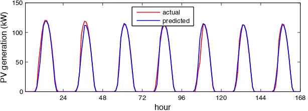
3.8 PV prediction . . . 45
3.9 Workload analysis and prediction . . . 46
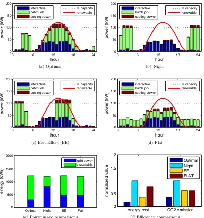
3.10 Power cost minimization while finishing all jobs . . . 49
3.11 Benefit of cooling integration . . . 50
3.12 Benefit of cooling optimization . . . 52
3.13 Net Zero Energy . . . 53
3.14 Optimal renewable portfolio . . . 54
3.15 Impact of PV prediction error . . . 55
3.17 Impact of workload characteristics . . . 55 3.18 Comparison of plan and experimental results . . . 57 3.19 Comparison of optimal and night . . . 58
4.1 Occurrence of coincident peak and warnings. (a) Empirical frequency of CP occurrences on the time of day, (b) Empirical frequency of CP occurrences over the week, (c) Empirical frequency of warning occurrences on the time of day, and (d) Empirical frequency of warning occurrences over the week. . . 64 4.2 Overview of warning occurrences showing (a) daily frequency, (b) length, and (c)-(d)
monthly frequency. . . 66 4.3 One week traces for (a) PV generation, (b) non-flexible workload demand, (c) flexible
workload demand, and (d) cooling efficiency. . . 67 4.4 Comparison of energy costs and emissions for a data center with a local PV installation
and a local diesel generator. (a)-(j) show the plans computed by our algorithms and the baselines. . . 79 4.5 Comparison of energy costs and emissions for a data center without local generation
or PV generation. (a)-(d) show the plans computed by our algorithms. . . 81 4.6 Comparison of energy costs and emissions for a data center with a local PV installation,
but without local generation. (a)-(d) show the plans computed by our algorithms. . . 82 4.7 Comparison of energy costs and emissions for a data center with a local diesel generator,
but without local PV generation. (a)-(d) show the plans computed by our algorithms. 83 4.8 Sensitivity analysis of “Prediction” and “Robust” algorithms with respect to (a)
work-load and renewable generation prediction error and (b) & (c) coincident peak and warning prediction errors. In all cases, the data center considered has a local diesel generator, but no local PV installation. . . 83
5.1 SCE 47 bus network. . . 89 5.2 SCE 56 bus network. . . 89 5.3 One week traces for (a) PV generation, (b) inflexible workload, (c) flexible workload,
and (d) cooling efficiency. . . 90 5.4 Impact of energy storage capacity,Cs, on the voltage violation rates. . . 93
5.5 Impact of energy storage charging rate on the voltage violation rates. . . 93 5.6 Diagram of the capacity of storage necessary to achieve the same voltage violation
5.7 Comparison of a 20MW data center to large-scale storage in a 47 bus SCE distribution network. (a)-(c) show the violation frequency as a function of the amount of data center flexibility,e, and compare to optimally placed storage, for different locations of the data center. (d) shows the violation frequency resulting from a data center with
e= 0.2 versus 0.33MWh of storage, for each location. . . 96 5.8 Comparison of a 4MW data center to large-scale storage in a 56 bus SCE
distribu-tion network. (a) shows the violadistribu-tion frequency as a funcdistribu-tion of the amount of data center flexibility,e, and compare to optimally placed storage. (b) shows the violation frequency resulting from a data center with e = 0.2 compared to 0.07MWh of storage at each location. . . 97 5.9 Comparison of a 20MW data center with a co-located 5MW PV installation to
large-scale storage in a 47 bus SCE distribution network. (a) depicts the data center located at bus 2. (b) shows the violation frequency resulting from a data center withe= 0.2 compared to 0.33MWh of storage, for each location. . . 98 5.10 Comparison of prediction-based pricing and supply function bidding demand response
programs. (a) shows the efficiency loss as a function of the prediction error withn= 5. (b) shows the prediction error at which prediction-based pricing begins to have worse efficiency than supply function bidding for eachn. . . 105
C.1 Illustration of pdf ofε(t) that attainsE[ε(t)+] = 1
2σε(t)forE[ε(t)] = 0 andV[ε(t)] =σ 2
ε(t).157
C.2 Instance for lower bounding the competitive ratio for setting with local generation. . . 158
List of Tables
Chapter 1
Introduction
This thesis aims to develop analytical models, deployable algorithms, and real systems to enable efficient integration of renewable energy into IT systems and furthermore, to use IT to improve the sustainability and efficiency of our broad energy infrastructure through data center demand response.
Data center demand response sits at the intersection of two important societal challenges. First, as IT becomes increasingly crucial to society, the associated energy demands skyrocket, e.g., within the US the growth in electricity demand of IT is ten times larger than the overall growth of elec-tricity demands [78, 160, 110]. Second, the integration of renewable energy into the power grid is fundamental for improving sustainability, but causes significant challenges for management of the grid that can potentially increase costs considerably [57, 63]. Further, this challenge is magnified by the fact that large-scale fast-charging storage is simply not cost-effective at this point.
The key idea behind data center demand response is that these two challenges are in fact symbi-otic. Specifically, data centers are large loads, but are also flexible – data center loads can often be shifted in time [70, 44, 120, 86, 132, 197, 193, 121], curtailed via quality degradation [20, 85, 180, 189], or even shifted geographically [150, 153, 184, 123, 122, 188, 119, 34]. If the flexibility of data centers can be called on by the grid via demand response programs, then they can be a crucial tool for eas-ing the incorporation of renewable energy into the grid. Further, this interaction can be “win-win” because the financial benefits from data center participation in demand response programs can help ease the burden of skyrocketing energy costs.
The first thrust of the thesis is to make IT systems more sustainable by facilitating the integration
44, 32], but the efficiency improvements do not necessarily lead to reduction in energy consumption because more servers are demanded as another instance of Jevons Paradox. Further, little effort has been put in making IT more sustainable, e.g., quite a lot of data centers are built at locations with cheap yet “dirty” electricity supply, and most of the improvements are from improved engineering rather than improved “algorithms”.
In contrast, this work focuses on developing algorithms with rigorous theoretical analysis that improve the sustainability of IT systems. In particular, this research seeks to exploit the flexibilities of cloud workloads both (i) in time by scheduling delay-tolerant workloads and (ii) in space by routing requests to geographically diverse data centers. These opportunities allow cloud data centers to adaptively respond to renewable availability, varying cooling efficiency, and fluctuating energy prices, while still meeting performance requirements, by performing the “geographical load balancing”. The design of the enabling algorithms is however highly challenging because of limited information, non-smoothness of objective functions, and the need of distributed control. Chapter 2 therefore focuses on these algorithmic challenges. In particular, three distributed algorithms are derived for achieving optimal geographical load balancing to enable the “follow the renewables” routing with theoretically guaranteed convergence to an optimal solution. Our real trace driven numerical simulations show that the “geographical load balancing”, if incentivized properly, can significantly reduce non-renewable energy usage and/or required capacity of renewable energy for the system to become sustainable. The work presented in this chapter is based on publication [123].
“optimization-based designs” recently proposed, e.g., [114, 123, 153, 184, 120, 143, 122, 119]. The work presented in this chapter is based on publication [121].
The second thrust of this thesis is to use IT systems to improve the sustainability and efficiency
of our broad energy infrastructure through data center demand response. The main challenges as we integrate more renewable sources to the existing power grid come from the fluctuation and unpredictability of renewable generation. Although energy storage and reserves can potentially solve the issues, they are very costly. One promising alternative is to make geographically distributed data centers demand responsive because it can provide significant peak demand reduction and ease the incorporation of renewable energy into the grid. The potential of such an approach is huge. The energy usage of cloud computing is estimated to grow at 20-30% annually over the coming decades, which nearly matches the estimated growth rate of wind and solar installments. Data centers has a huge potential to provide a large fraction of the amount of storage needed to incorporate renewable resources smoothly.
To realize this potential, we need adaptive and distributed control of cloud data centers and new electricity market designs for distributed electricity resources. My work is progressing in both directions. Chapter 4 focuses on the design of local algorithms. In particular, we study two demand response schemes to reduce a data center’s peak loads and energy expenditure: workload shifting and the use of local power generation in coincident peak pricing program [67]. We develop a detailed characterization of coincident peak data over two decades from Fort Collins Utilities, Colorado and then design two algorithms for data centers by combining workload scheduling and local power generation to avoid the coincident peak and reduce energy expenditure. The first algorithm optimizes the expected cost and the second provides a good worst-case guarantee for any coincident peak pattern, workload demand and renewable generation prediction error distributions. We evaluate these algorithms via numerical simulations based on real world traces from production systems. The results show that using workload shifting in combination with local generation can provide significant cost savings compared to either alone. The work presented in this chapter is based on publication [125].
Chapter 2
Sustainable IT: Greening
Geographical Load Balancing
Increasingly web services are provided by massive, geographically diverse “Internet-scale” distributed systems, some having several data centers each with hundreds of thousands of servers. Such data centers require many megawatts of electricity and so companies like Google and Microsoft pay tens of millions of dollars annually for electricity [150].
The enormous, and growing, energy demands of data centers have motivated research both in academia and industry on reducing energy usage, for both economic and environmental reasons. Engineering advances in cooling, virtualization, DC power, etc. have led to significant improvements in the Power Usage Effectiveness (PUE) of data centers; see [24, 170, 102, 107]. Such work focuses on reducing theenergy use of data centers and their components.
A different stream of research has focused on exploiting the geographical diversity of Internet-scale systems to reduce theenergy cost. Specifically, a system with clusters at tens or hundreds of locations around the world can dynamically route requests/jobs to clusters based on proximity to the user, load, and local electricity price. Thus, dynamic geographical load balancing can balance the revenue lost due to increased delay against the electricity costs at each location.
The potential of geographical load balancing to provide significant cost savings for data centers is well known; see [114, 143, 150, 153, 165, 184] and the references therein. The goal of the current work is different. Our goal is to explore the social impact of geographical load balancing systems. In particular, because GLB reduces the average price of electricity, it reduces the incentive to make other energy-saving tradeoffs.
the prohibitive cost of high-capacity long-distance electricity transmission lines), renewable sources pose a significant challenge. A key technique for handling the non-dispatchability of renewable sources is demand response, which entails the grid adjusting the demand by changing the electric-ity price [8]. However, demand response entails a local customer curtailing use. In contrast, the demand of Internet-scale systems is flexible geographically; thus requests can be routed to different regions to “follow the renewables” to do the work in the right place, providing demand response without service interruption. Since data centers represent a significant and rapidly growing fraction of total electricity consumption, and the IT infrastructure with necessary knobs is already in place, geographical load balancing can provide an inexpensive approach for enabling large scale, global demand response.
The key to realizing the environmental benefits above is for data centers to move from the typical fixed price contracts that are now widely used toward some degree of dynamic pricing, with lower prices when renewable energy generation exceeds expectation. The current demand response markets provide a natural way for this transition to occur, and there is already evidence of some data centers participating in such markets [1].
The contribution of this chapter is twofold. (1) We develop distributed algorithms for geograph-ical load balancing with provable optimality guarantees. (2) We use the proposed algorithms to explore the feasibility and consequences of using geographical load balancing for demand response in the grid.
Contribution (1): To derive distributed geographical load balancing algorithms we use a simple but general model, described in detail in Section 2.1. In it, each data center minimizes its cost, which is a linear combination of an energy cost and the lost revenue due to the delay of requests (which includes both network propagation delay and load-dependent queueing delay within a data center). The geographical load balancing algorithm must then dynamically decide both how requests should be routed to data centers and how to allocate capacity in each data center (e.g., speed scaling and how many servers are kept in active/energy-saving states).
In Section 2.2, we characterize the optimal geographical load balancing solutions and show that they have practically appealing properties, such as sparse routing tables. In Section 2.3, we use the previous characterization to design three distributed algorithms which provably compute the optimal routing and provisioning decisions and require different degrees of coordination. The key challenge here is how to design distributed algorithms with guaranteed convergence without Lipschitz continuity. Finally, we evaluate the distributed algorithms using numeric simulation of a realistic, distributed, Internet-scale system (Section 2.4). The results show that a cost saving of over 40% during light-traffic periods is possible.
trace-driven numeric simulation of a realistic, distributed Internet-scale system in combination with real wind and solar energy generation traces over time.
When the data center incentive is aligned with the social objective for reducing brown energy by dynamically pricing electricity proportionally to the fraction of the total energy coming from brown sources, we show that “follow the renewables” routing ensues (see Figure 2.5), providing significant social benefit. We determine the wasted brown energy when prices are static, or are dynamic but do not align data center and social objectives enough, also later shown by [72].
2.1
Model and Notation
We now introduce the workload and data center models, followed by the geographical load balancing problem.
2.1.1
The workload model
We consider a discrete-time model with time step duration normalized to 1, such that routing and capacity provisioning decisions can be updated within a time slot. There is a (possibly long) interval of interestt∈ {1, . . . , T}. There are|J|geographically concentrated sources of requests, i.e., “cities”, and work consists of jobs that arrive at a mean arrival rate ofLj(t) from sourcej at timetis. Jobs
are assumed to be small, so that provisioning can be based on the Lj(t). In practice,T could be a
month and a timeslot length could be 1 hour. Our analytic results make no assumptions onLj(t);
however numerical results in Sections 2.4 and 2.5 use measured traces to defineLj(t).
2.1.2
The data center cost model
We model an Internet-scale system as a collection of|N|geographically diverse data centers, where data centeriis modeled as a collection of Mi homogeneous servers. The model focuses on two key
control decisions of geographical load balancing at each timet: (i) determining λij(t), the amount
of requests routed from source j to data center i; and (ii) determining mi(t) ∈ {0, . . . , Mi}, the
number of active servers at data centeri. Since Internet data centers typically contain thousands of active servers, we neglect the integrality constraint on mi. The system seeks to chooseλij(t) and
mi(t) in order to minimize cost during [1, T]. Depending on the system design, these decisions may
be centralized or decentralized. Section 2.3 focuses on the algorithms for this.
Our model for data center costs focuses on the server costs of the data center.1 We model costs
by combining the energy cost and thedelay cost (in terms of lost revenue). Note that, to simplify the model, we do not include the switching costs associated with cycling servers in and out of
saving modes; however, the approach of [119, 120] provides a natural way to incorporate such costs if desired.
Energy cost. To capture the geographical diversity and variation over time of energy costs, we letgi(t, mi, λi) denote the energy cost for data centeriduring timeslottgivenmi active servers and
arrival rateλi including cooling power [161, 113, 121]. For every fixedt, we assume thatgi(t, mi, λi)
is continuously differentiable in bothmi andλi, strictly increasing inmi, non-decreasing inλi, and
jointly convex in mi and λi. This formulation is quite general. It can capture a wide range of
models for power consumption, e.g., energy costs as an affine function of the load, see [62], or as a polynomial function of the speed, see [185, 19]2.
Definingλi(t) =Pj∈Jλij(t),∀t, the total energy cost of data centeriduring timeslott, denoted
byEi(t), is simply
Ei(t) =gi(t, mi(t), λi(t)). (2.1)
Delay cost. The delay cost captures the lost revenue incurred from the delay experienced by the requests. To model this, we definer(d) as the lost revenue associated with average delay d. We assume thatr(d) is strictly increasing and convex ind.
We consider the two components of delay: the network delay while the request is outside the data center and the queueing delay within the data center. To model delay, we consider its two components: the network delay experienced while the request is outside of the data center and the queueing delay experienced in the data center.
Letdij(t) denote the averagenetwork delay of requests from sourcejto data centeriin timeslot
t. Letfi(mi, λi) be the average queueing delay at data centerigivenmiactive servers and an arrival
rate ofλi. We assume thatfiis strictly decreasing inmi, strictly increasing inλi, and strictly convex
in both mi and λi. Further, for stability, we must have that λi = 0 or λi < miµi, whereµi is the
service rate of a server at data centeri. Thus, we definefi(mi, λi) =∞ forλi ≥miµi. For other
mi, we assume fi is finite, continuous and differentiable. Note that these assumptions are satisfied
by most standard queueing formula, e.g., the average delay under M/GI/1 Processor Sharing (PS) queue and the 95th percentile of delay under the M/M/1. Further, the convexity offiinmi models
the law of diminishing returns for parallelism.
Combining the above gives the following model for the total delay cost Di(t) at data center i
during timeslott:
Di(t) =
X
j∈Jλij(t)r
fi(mi(t), λi(t)) +dij(t)
. (2.2)
2We focus on the issue of peak pricing in our recent work [125]. It requires slightly different approaches, but they
2.1.3
The geographical load balancing problem
Given the cost models above, the goal of geographical load balancing is to choose the routing policy
λij(t) and the number of active servers in each data center mi(t) at each timet in order minimize
the total cost during [1, T]. This is captured by the following optimization problem:
min
m(t),λ(t)
XT
t=1
X
i∈N(Ei(t) +Di(t)) (2.3a)
s.t. X
i∈Nλij(t) =Lj(t), ∀j ∈J (2.3b)
λij(t)≥0, ∀i∈N,∀j ∈J (2.3c)
0≤mi(t)≤Mi, ∀i∈N (2.3d)
mi(t)∈N, ∀i∈N (2.3e)
So, we can relax the integer constraint in (2.3) and round the resulting solution with minimal increase in cost. Because this model neglects the cost of turning servers on and off, the optimization decouples into independent sub-problems for each timeslot t. For the analysis we consider only a single interval.3 Thus, the minimization of the aggregate ofE
i(t) +Di(i) is achieved by solving, at
each timeslot,
min
m,λ
X
i∈N
gi(mi, λi) +
X
i∈N
X
j∈J
λijr(dij+fi(mi, λi)) (2.4a)
s.t. X
i∈Nλij =Lj, ∀j∈J (2.4b)
λij ≥0, ∀i∈N,∀j∈J (2.4c)
0≤mi≤Mi, ∀i∈N. (2.4d)
where m = (mi)i∈N and λ= (λij)i∈N,j∈J. We refer to this formulation as GLB. Note that GLB
is jointly convex in λij and mi and can be efficiently solved centrally[31]. However, a distributed
solution algorithm is usually required by large-scale systems, such as those derived in Section 2.3. In contrast to prior work on geographical load balancing, this work jointly optimizes total energy cost and end-to-end user delay, with consideration of both price and network delay diversity. To our knowledge, this is the first work to do so.
GLB provides a general framework for studying geographical load balancing. However, the model still ignores many aspects of data center design, e.g., reliability and availability, which are central
3Time-dependence ofL
to data center service level agreements. Such issues are beyond the scope of this work; however our designs merge nicely with proposals such as [168] for these goals.
The GLB model is too broad for some of our analytic results and thus we often use two restricted versions.
Linear lost revenue. There is evidence that lost revenue is linear within the range of interest for sites such as Google, Bing, and Shopzilla [52, 2]. To model this, we can let r(d) = βd, for constantβ. GLB then simplifies to
min
subject to (2.4b)–(2.4d). We call this optimization GLB-LIN.
Queueing-based delay. We occasionally specify the form of f andg using queueing models. This provides increased intuitions about the distributed algorithms presented.
If the workload is perfectly parallelizable, and arrivals are Poisson, thenfi(mi, λi) is the average
delay ofmiparallel queues, with arrival rateλi/mi. Moreover, if each queue is an M/GI/1 PS queue,
fi(mi, λi) = 1/(µi−λi/mi). We also assumegi(mi, λi) =pimi, which implies that the increase in
energy cost per timeslot for being in an active state, rather than a low-power state, ismi regardless
ofλi. Note that cooling efficiency of data centerican be integrated inpi, which allows incorporation
of cooling power consumption.
Under these restrictions, the GLB formulation becomes:
min
subject to (2.4b)–(2.4d) and the additional constraint
λi≤miµi ∀i∈N. (2.6b)
We refer to this optimization as GLB-Q.
Additional Notation. Throughout the chapter we use|S|to denote the cardinality of a setS
2.1.4
Practical considerations
Our model assumes there exist mechanisms for dynamically (i) provisioning capacity of data cen-ters, and (ii) adapting the routing of requests from sources to data centers. With respect to (i), many dynamic server provisioning techniques are being explored by both academics and industry, e.g., [16, 43, 71, 173]. With respect to (ii), there are also a variety of protocol-level mechanisms employed for data center selection today. They include, (a) dynamically generated DNS responses, (b) HTTP redirection, and (c) using persistent HTTP proxies to tunnel requests. Each of these has been evaluated thoroughly, e.g., [49, 131, 146, 184], and though DNS has drawbacks it remains the preferred mechanism for many industry leaders such as Akamai, possibly due to the added latency due to HTTP redirection and tunneling [144]. Within the GLB model, we have implicitly assumed that there exists a proxy/DNS server co-located with each source. The practicality is also shown by [78]. Our model also assumes that the network delays,dij can be estimated, which has been studied
extensively, including work on reducing the overhead of such measurements, e.g., [167], and mapping and synthetic coordinate approaches, e.g., [111, 141]. We discuss the sensitivity of our algorithms to error in these estimates in Section 2.4.
2.2
Characterizing the optima
We now provide characterizations of the optimal solutions to GLB, which are important for proving convergence of the distributed algorithms in Section 2.3. They are also necessary because, a priori, one might worry that the optimal solution requires a very complex routing structure, which would be impractical; or that the set of optimal solutions is very fragmented, which would slow convergence in practice. The results here show that such worries are unwarranted.
Uniqueness of optimal solution
To begin, note that GLB has at least one optimal solution. This can be seen by applying Weierstrass’ theorem [25], since the objective function is continuous and the feasible set is compact subset ofRn.
Although the optimal solution is generally not unique, there are natural aggregate quantities unique over the set of optimal solutions, which is a convex set. These are the focus of this section.
A first result is that for the GLB-LIN formulation, under weak conditions on fi andgi, we have
that λi is common across all optimal solutions. Thus, the input to the data center provisioning
optimization is unique.
Theorem 1. Consider the GLB-LIN formulation. Suppose that for alli,Fi(mi, λi)is jointly convex
inλi andmi, and continuously differentiable in λi. Further, suppose thatmˆi(λi)is strictly convex.
The proofs of this subsection are in the Appendix A.2. Note that theorem 1 implies that the server arrival rates at each data center, i.e.,λi/mi, are common among all optimal solutions.
Though the conditions onFi and ˆmiare weak, they do not hold for GLB-Q. In that case, ˆmi(λi)
is linear, and thus not strictly convex. Although theλi are not common across all optimal solutions
in this setting, the server arrival rates remain common across all optimal solutions.
Theorem 2. For each data centeri, the server arrival rates,λi/mi, are common across all optimal
solutions to GLB-Q.
Sparsity of routing
It would be impractical if the optimal solutions to GLB required that requests from each source were divided up among (nearly) all of the data centers. In general, eachλij could be non-zero, yielding
|N|×|J|flows of requests from sources to data centers, which would lead to significant scaling issues. Luckily, there is guaranteed to exist an optimal solution with extremely sparse routing. Specifically, we have the following result.
Theorem 3. There exists an optimal solution to GLB with at most(|N|+|J| −1)of theλij strictly
positive.
Though Theorem 3 does not guarantee that every optimal solution is sparse, the proof is con-structive. Thus, it provides an approach which allows one to transform any optimal solution into a sparse optimal one.
The following result further highlights the sparsity of the routing: any source will route to at most one data center that is not fully active, i.e., where there exists at least one server in power-saving mode.
Theorem 4. Consider GLB-Q where power costs pi are drawn from an arbitrary continuous
dis-tribution. If any source j ∈ J has its requests split between multiple data centers N0 ⊆N in an
optimal solution, then, with probability 1, at most one data centeri∈N0 has mi< Mi.
2.3
Algorithms
We now present three distributed algorithms and prove their convergence. For simplicity we focus on GLB-Q; the approaches are applicable more generally, but become much more complex for richer models.
systems to outsource route selection [184]. To meet this need, the algorithms presented below are decentralized and allow each data center and proxy to optimize based on partial information.
These algorithms seek to fill a notable gap in the growing literature on algorithms for geographical load balancing. Specifically, they have provable optimality guarantees for a performance objective that includes both energy and delay, where route decisions are made using energy price and network propagation delay information. The most closely related work [153] investigates the total electricity cost for data centers in a multi-electricity-market environment. It contains the queueing delay inside the data center (assumed to be a centralizedM/M/1 queue), but neglects the end-to-end user delay. Conversely, [184] uses a simple, efficient algorithm to coordinate the “replica-selection” decisions for load balancing. Other related works, e.g., [153, 150, 143], either do not provide provable guarantees or ignore diverse network delays and/or prices.
Algorithm 1: Gauss-Seidel iteration
Algorithm 1 is motivated by the observation that GLB-Q is separable in mi, and, less obviously,
also separable in λj := (λij, i ∈N). This allows all data centers as a group and each proxy j to
iteratively solve for optimalmandλjin a distributed manner, and communicate their intermediate
results. Though distributed, Algorithm 1 requires each proxy to solve an optimization problem. To highlight the separation between data centers and proxies, we reformulate GLB-Q as:
min
Since the objective and constraintsMi and Λj are separable, this can be solved separately by data
centersiand proxiesj.
proxyj depends onλ−j only through their aggregate arrival rates at data centers:
subtracting its ownλij(τ) from the value received from data centeri. This has less overhead than
direct messaging.
In summary, Algorithm 1 works as follows (note that the minimization (2.9) has a closed form). Here, [x]a := min{x, a}.
Algorithm 1. Starting from a feasible initial allocationλ(0) and the associatedm(λ(0)), let
mi(τ+ 1) :=
Since GLB-Q generally has multiple optimal λ∗j, Algorithm 1 is not guaranteed to converge to one particular optimal solution, i.e., for each proxyj, the allocationλij(τ) of jobjto data centersi
may oscillate among multiple optimal allocations. However, both the optimal cost and the optimal per-server arrival rates to data centers will converge.
Theorem 5. Let (m(τ),λ(τ)) be a sequence generated by Algorithm 1 when applied to GLB-Q.
The proof of Theorem 5 follows from the fact that Algorithm 1 is a modified Gauss-Seidel iteration. This is also the reason for the requirement that the proxies update sequentially. The details of the proof are in Appendix A.3.
using possibly outdated information. The algorithm generalizes easily to this setting, though the convergence proof is more difficult. The convergence rate of Algorithm 1 in a realistic scenario is illustrated numerically in Section 2.4.
Algorithm 2: Distributed gradient projection
Algorithm 2 reduces the computational load on the proxies. In each iteration, instead of each proxy solving a constrained minimization (2.12) as in Algorithm 1, Algorithm 2 takes a single step in a descent direction. Also, while the proxies compute their λj(τ + 1) sequentially in |J| phases in
Algorithm 1, they perform their updates all at once in Algorithm 2. To achieve this, rewrite GLB-Q as
min
definition of Algorithm 1, this minimization is easy: if we denote the solution to (2.11) by
mi(λi) :=
We now sketch the two key ideas behind Algorithm 2. The first is the standard gradient projection idea: move in the steepest descent direction
−∇Fj(λ) :=−
and then project the new point into the feasible set Q
jΛj with Λj given by (2.8). The standard
gradient projection algorithm will converge if∇F(λ) is Lipschitz overQ
jΛj. This condition,
how-ever, does not hold for ourF because of the termβλi/(µi−λi/mi). The second idea is to construct
a compact and convex subset Λ of the feasible set Q
jΛj with the following properties: (i) if the
algorithm starts in Λ, it stays in Λ; (ii) Λ contains all optimal allocations; (iii)∇F(λ) is Lipschitz over Λ. The algorithm then projects into Λ in each iteration instead of Q
jΛj. This guarantees
convergence.
Specifically, fix a feasible initial allocation λ(0) ∈ Q
objective value. Define
Even though the Λ defined in (2.15) indeed has the desired properties (see Appendix A.4), the projection into Λ requires coordination of all proxies and is thus impractical. In order for each proxy
j to perform its update in a decentralized manner, we define proxyj’s own constraint subset:
ˆ
data center i’s measured arrival rates λi(τ), as done in Algorithm 1 in (2.10) and the discussion
thereafter, and does not need to communicate with other proxies. Hence, givenλi(τ,−j) from data
centersi, each proxy can project into ˆΛj(τ) to compute the next iterateλj(τ+ 1) without the need
to coordinate with other proxies.4 Moreover, ifλ(0)∈Λ thenλ(τ)∈Λ for all iterationsτ.
Algorithm 2. Starting from a feasible initial allocation λ(0) and the associated m(λ(0)), each proxyj computes, in each iterationτ:
zj(τ+ 1) := [λj(τ)−γj(∇Fj(λ(τ)))]Λˆ
Algorithm 2 has the same convergence property as Algorithm 1, provided the stepsize is small enough.
4The projection to the nearest point in ˆΛ
Theorem 6 is proven in Appendix A.4. The key novelty of the proof is (i) handling the fact that the objective is not Lipshitz and (ii) allowing distributed computation of the projection. The bound onγj in Theorem 6 is more conservative than necessary for large systems. Hence, a larger stepsize
can be choosen to accelerate convergence. The convergence rate is illustrated in a realistic setting in Section 2.4.
Algorithm 3: Distributed Gradient Descent
Like Algorithm 2, Algorithm 3 is a gradient-based algorithm. The key distinction is that Algorithm 3 avoids the need for projection in each iteration, based on two ideas. First, instead of moving in the steepest descent direction, each proxyj re-distributes its jobs among data centers so thatP
iλij(τ)
always equals toLj in each iterationτ. Second, instead of a constant stepsize, Algorithm 3 carefully
adjusts a time-varying stepsize in each iteration to ensure that the new allocation is feasible without the need for projection. The design of the stepsize must be such that each proxy j can set its ownγj(τ) in iteration τ using only local information. Moreover,γj(τ) must ensure: (i) collectively
λ(τ+ 1) must stay in the set Λ0 over which∇F is Lipschitz; (ii)λ(τ+ 1)≥0; and (iii) F(λ(τ)) decreases sufficiently in each iteration. Define
Λ0:= Λ0(φ) = ΠjΛj∩
be the set of data centers that either are allocated significant amount of data, i.e., larger than , from j in round τ or will receive an increased allocation from j in round τ+ 1, i.e., those with a gradient less thanx. Then let
be the maximum step size for which no data center will be reduced to an allocation below 0 and
be a lower bound on the maximum step size for which no data center will have its load increased beyond that permitted by Λ0j(τ). Algorithm 3 proceeds as follows.
Algorithm 3. Let K0 = maxi
16|J|(φ+βMi)3
β2M4 iµ2i
. Select % ∈ (0,2). Starting from a feasible initial allocation λ(0), each proxyj computes, in each iterationτ:
γj(τ) := min
As in the case of Algorithm 2, implicit in the description is the requirement that all data centers
icomputemi(λi(τ)) according to (2.14) in each iterationτ. The procedure for this is the same as
discussed for Algorithm 2.
Theorem 7. When using Algorithm 3 in the GLB-Q formulation,F(λ(τ))converges to a value no greater than optimal value plusB, whereB =β|J|P
Also, as with Algorithm 2, the key novelty of the proof of Theorem 7 is the fact that we can prove convergence even though the objective function is not Lipschitz. The proof of Theorem 7 is provided in Appendix A.5. Finally, note that the convergence rate of Algorithm 3 is even faster than that of Algorithm 2 in realistic settings, as we illustrate in Section 2.4. We can consider as the tolerant of error when the optimal allocationλij= 0. In practice, we can setto a small value,
then Algorithm 3 willalmost converge to the optimal value.
2.4
Case study
12 24 36 48 0
0.05 0.1 0.15 0.2
time(hour)
arrival rate
(a) Original trace
12 24 36 48
0 0.05 0.1 0.15 0.2
time(hour)
arrival rate
(b) Adjusted trace
Figure 2.1: Hotmail trace used in numerical results.
2.4.1
Experimental setup
We aim to use realistic parameters in the experimental setup and provide conservative estimates of the cost savings resulting from optimal geographical load balancing. The setup models an Internet-scale system such as Google within the United States.
Workload description
1 1.5 2 2.5 x 10⁵ 4
5 6 7 8 9x 10
4
delay
energy cost
t=7am t=8am t=9am
Figure 2.2: Pareto frontier of the GLB-Q formulation as a function of β for three different times (and thus arrival rates), PDT. Circles, x-marks, and triangles correspond to β = 0.4, 1, and 2.5, respectively.
Data center description
To model an Internet-scale system, we have 14 data centers, one at the geographic center of each state known to have Google data centers [94]: California, Washington, Oregon, Illinois, Georgia, Virginia, Texas, Florida, North Carolina, and South Carolina.
We merge the data centers in each state and set Mi proportional to the number of data centers
in that state, while keeping Σi∈NMiµi twice the total peak workload, maxtΣj∈JLj(t). The network
delays, dij, between sources and data centers are taken to be proportional to the geographical
distances between them and comparable to the average queueing delays inside the data centers. This lower bound on the network delay ignores delay due to congestion or indirect routes.
Cost function parameters
To model the costs of the system, we use the GLB-Q formulation. We setµi = 1 for all i, so that
0 100 200 300 400 500 0
5 10 15
x 104
time(slot)
cost
Algorithm 1 Algorithm 2 Algorithm 3 Optimal
(a) Static setting
1000 2000 3000 4000 5000 6000 7000 0
5 10 15x 10
4
phase
cost
Algorithm 1 Optimal
(b) Dynamic setting
Figure 2.3: Convergence of all three algorithms.
Algorithm benchmarks
To provide benchmarks for the performance of the algorithms presented here, we consider three baselines, which are approximations of common approaches used in Internet-scale systems. They also allow implicit comparisons with prior work such as [153]. The approaches use different amounts of information to perform the cost minimization. Note that each approach must use queueing delay (or capacity information); otherwise the routing may lead to instability.
Baseline 1 uses network delays, but ignores energy price when minimizing its costs. This demon-strates the impact of price-aware routing. It also shows the importance of dynamic capacity provi-sioning, since without using energy cost in the optimization, every data center will keep every server active.
Baseline 2 uses energy prices, but ignores network delay. This illustrates the impact of location-aware routing on the data center costs. Further, it allows us to understand the performance im-provement of our algorithms compared to those such as [153, 165] that neglect network delays in their formulations.
Baseline 3 uses neither network delay information nor energy price information when performing its cost minimization. Thus, the traffic is routed so as to balance the delays within data centers. Though naive, designs such as this are still used by systems today; see [10].
2.4.2
Performance evaluation
Convergence
We start by considering the convergence of each of the distributed algorithms. Figure 2.3(a) illus-trates the convergence of each of the algorithms in a static setting for t = 11am, where load and electricity prices are fixed and each phase in Algorithm 1 is considered as an iteration. It validates the convergence analysis for both algorithms. Note here Algorithm 2 and Algorithm 3 use a step size
γ= 10; this is much larger than that used in the convergence analysis, which is quite conservative, and there is no sign of causing lack of convergence.
To demonstrate the convergence in a dynamic setting, Figure 2.3(b) shows Algorithm 1’s re-sponse to the first day of the Hotmail trace, with loads averaged over one-hour intervals for brevity. One iteration is performed every 10 minutes. This figure shows that even the slower algorithm, Algorithm 1, converges fast enough to provide near-optimal cost. Hence, the remaining plots show only the optimal solution.
Energy versus delay tradeoff
The optimization objective we have chosen to model the data center costs imposes a particular tradeoff between the delay and the energy costs,β. It is important to understand the impact of this factor. Figure 2.2 illustrates how the delay and energy cost trade off under the optimal solution asβ
changes. Thus, the plot shows the Pareto frontier for the GLB-Q formulation. The figure highlights that there is a smooth convex frontier with a mild ‘knee’.
Cost savings
To evaluate the cost savings of geographical load balancing, Figure 2.4 compares the optimal costs to those incurred under the three baseline strategies described in the experimental setup. The overall cost, shown in Figures 2.4(a) and 2.4(b), is significantly lower under the optimal solution than all of the baselines (nearly 40% during times of light traffic). Recall that Baseline 2 is the state of the art, studied in recent papers such as [153, 165].
12 24 36 48
(b) Total cost (% improvement vs. Baseline 3)
12 24 36 48
Figure 2.4: Impact of ignoring network delay and/or energy price on the cost incurred by geographical load balancing.
network delay is not considered, a proxy is more likely to route to a data center that is not yet running at full capacity, thereby adding to the energy cost.
Sensitivity analysis
We have studied the sensitivity of the algorithms to errors in the inputs loadLj and network delay
dij. Estimation errors inLj only affect the routing. In our model data centers adapt their number
of servers based on the true load, which counteracts suboptimal routing. In our context, network delay was 15% of the cost, and so large relative errors in delay had little impact. Baseline 2 can be thought of as applying the optimal algorithm to extremely poor estimates of dij (namelydij = 0),
2.5
Social impact
We now shift focus from the cost savings of the data center operator to the social impact of geo-graphical load balancing. We focus on the impact of geogeo-graphical load balancing on the usage of “brown” non-renewable energy by Internet-scale systems, and how this impact depends on electricity pricing.
Intuitively, geographical load balancing allows the traffic to “follow the renewables”; thus pro-viding increased usage of green energy and decreased brown energy usage. However, such benefits are only possible if data centers forgo static energy contracts for dynamic energy pricing (either through demand response programs or real-time pricing). The experiments in this section show that if dynamic pricing is done optimally, then geographical load balancing can provide significant social benefits by reducing non-renewable energy consumption.
2.5.1
Experimental setup
To explore the social impact of geographical load balancing, we use the setup described in Section 2.4. However, we add models for the availability of renewable energy, the pricing of renewable energy, and the social objective.
The availability of renewable energy
To capture the availability of wind and solar energy, we use traces of wind speed and Global Hori-zontal Irradiance (GHI) obtained from [90, 92] that have measurements every 10 minutes for a year. The normalized generations of four states (CA, TX, IL, NC) and the West/East Coast average are illustrated in Figure 2.5(a), where 50% of renewable energy comes from solar.
Building on these availability traces, for each location we let αi(t) denote the fraction of the
energy that is from renewable sources at time t, and let ¯α = (|N|T)−1PT
t=1
P
i∈Nαi(t) be the
“penetration” of renewable energy. We take ¯α = 0.30, which is on the progressive side of the renewable targets among US states [36].
Finally, when measuring the brown/green energy usage of a data center at timet, we use simply P
i∈Nαi(t)mi(t) as the green energy usage andPi∈N(1−αi(t))mi(t) as the brown energy usage.
This models the fact that the grid cannot differentiate the source of the electricity provided.
Dynamic pricing and demand response
To provide a simple model of demand response, we use time-varying pricespi(t) in each time-slot
that depend on the availability of renewable resourcesαi(t) in each location.
The way pi(t) is chosen as a function ofαi(t) will be of fundamental importance to the social
impact of geographical load balancing. To highlight this, we consider a parameterized “differentiated pricing” model that uses a pricepb for brown energy and a pricepg for green energy. Specifically,
pi(t) =pb(1−αi(t)) +pgαi(t).
Note that pg =pb corresponds to static pricing, and we show in the next section thatpg = 0
corresponds to socially optimal pricing. Our experiments varypg ∈[0, pb]. pb is the same price as
used in Section 2.4.
The social objective
To model the social impact of geographical load balancing we need to formulate a social objective. Like the GLB formulation, this must include a tradeoff between the energy usage and the average delay users of the system experience, because purely minimizing brown energy use requires all
mi= 0. The key difference between the GLB formulation and the social formulation is that thecost
of energy is no longer relevant. Instead, the environmental impact is important, and thus the brown energy usage should be minimized. This leads to the following simple model for the social objective:
min
m(t),λ(t)
T
X
t=1
X
i∈N
(1−αi(t))
Ei(t)
pi(t)
+ ˜βDi(t)
(2.21)
whereDi(t) is the delay cost defined in (2.2),Ei(t) is the energy cost defined in (2.1), and ˜β is the
relative valuation of delay versus energy. Further, we have imposed that the energy cost follows from the pricing ofpi(t) cents/kWh in timeslot t. Note that, though simple, our choice ofDi(t) to
model the disutility of delay to users is reasonable because lost revenue captures the lack of use as a function of increased delay.
An immediate observation about the above social objective is that to align the data center and social goals, one needs to set pi(t) = (1−αi(t))/β˜, which corresponds to choosing pb = 1/β˜ and
pg= 0 in the differentiated pricing model above. We refer to this as the “optimal” pricing model.
2.5.2
The importance of dynamic pricing
6 12 18 24 30 36 42 48
Figure 2.5: Geographical load balancing “following the renewables”. (a) Renewable availability. (b) and (c): Capacity provisionings of east coast and west coast data centers when there are renewables, under (b) optimal dynamic pricing and (c) static pricing. (d) Reduction in social cost from dynamic pricing compared to static pricing as a function of the weight for brown energy usage, 1/β˜, and
˜
β= 0.1.
service capacity from the west coast to the east coast as solar energy becomes highly available in the east coast and then switch back when solar energy is less available in the east coast, but high in the west coast. Though not explicit in the figures, this “follow the renewables” routing has the benefit of significantly reducing the brown energy usage since energy use is more correlated with the availability of renewables. Thus, geographical load balancing provides the opportunity to aid the incorporation of renewables into the grid.
[72]. Thus, it is important to consider the impact of partial adoption of dynamic pricing in addition to full, optimal dynamic pricing. Figure 2.5(d) focuses on this issue. To model the partial adoption of dynamic pricing, we can consider pg ∈ [0, pb]. This figure shows that the benefits provided by
dynamic pricing are moderate but significant, even at partial adoption (highpg). Another interesting
observation about Figure 2.5(d) is that the curves increase faster in the range when 1/β˜ is small, which highlights that the social benefit of geographical load balancing becomes significant even when there is only moderate importance placed on energy. Whenpg is higher thanpb, which is common
currently, the cost increases and geographical load balancing can no longer help to reduce non-renewable energy consumption. We omit the results due to space considerations. For more recent results about geographical load balancing in Internet-scale systems with local renewable generation and data center demand response to utility coincident peak charging, please refer to [122, 125].
2.6
Summary
Chapter 3
Sustainable IT: System Design and
Implementation
Data centers are emerging as the “factories” of this generation. A single data center requires a considerable amount of electricity and data centers are proliferating worldwide as a result of increased demand for IT applications and services. As a result, concerns about the growth in energy usage and emissions have led to social interest in curbing their energy consumption. These concerns have led to research efforts in both industry and academia. Emerging solutions include the incorporation of renewable on-site energy supplies as in Apple’s new North Carolina data center, and alternative cooling supplies as in Yahoo’s New York data center. The problem addressed by this chapter is how to use these resources most effectively during the operation of data centers.
Most of the efforts toward this goal focus on improving the efficiency in one of the three major data center silos: (i) IT, (ii) cooling, and (iii) power. Significant progress has been made in optimizing the energy efficiency of each of the three silos enabling sizeable reductions in data center energy usage, e.g., [62, 71, 120, 185, 104, 151, 183, 23]; however, the integration of these silos is an important next step. To this end, a second generation of solutions has begun to emerge. This work focuses on the integration of different silos [101, 137, 143, 44]. An example is the dynamic thermal management of air-conditioners based on load at the IT rack level [101, 32]. However, to this point, supply-side constraints such as renewable energy and cooling availability are largely treated independently from workload management such like scheduling. Particularly, current workload management are not designed to take advantage of time variations in renewable energy availability and cooling efficiencies. The work in [80] integrates power capping and consolidation with renewable energy, but they do not shift workloads to align power demand with renewable supply.
following three observations:
First, most data centers support a range of IT workloads, including both critical interactive applications that run 24x7 such like Internet services, and delay tolerant, batch-style applications as scientific applications, financial analysis, and image processing, which we refer to as batch workloads or batch jobs. Generally, batch workloads can be scheduled to run anytime as long as they finish before deadlines. This enables significant flexibility for workload management.
Second, the availability and cost of power supply, e.g., renewable energy supply and electricity price, is often dynamic over time, and so dynamic control of the supply mix can help reduce CO2
emissions and offset costs. Thus, thoughtful workload management can have a great impact on energy usage and costs by scheduling batch workloads in a manner that follows the renewable availability.
Third, many data centers nowadays are cooled by multiple means through a cooling micro grid combining traditional mechanical chillers, airside economizers, and waterside economizers. Within a micro grid, each cooling approach has a different efficiency and capacity that depends on IT workload, cooling generation mechanism and external conditions including outside air temperature and humidity, and may vary with the time of day. This provides opportunities to optimize cooling cost by “shaping” IT demand according to time varying cooling efficiency and capacity.
The three observations above highlight that there is considerable potential for integrated man-agement of the IT, cooling, and power subsystems of data centers. Providing such an integrated solution is the goal of this work. Specifically, we provide a novel workload scheduling and capac-ity management approach that integrates energy supply (renewable energy supply, dynamic energy pricing) and cooling supply (chiller cooling, outside air cooling) into IT workload management to improve the overall energy efficiency and reduce the carbon footprint of data center operations.
A key component of our approach is demand shifting, which schedules batch workloads and allocates IT resources within a data center according to the availability of renewable energy supply and the efficiency of cooling. This is a complex optimization problem due to the dynamism in the supply and demand and the interaction between them. To see this, given the lower electricity price and temperature of outside air at night, batch jobs should be scheduled to run at night; however, because more renewable energy like solar is available around noon, we should do more work during the day to reduce electricity bill and environmental impact.
IT Power
workloads; and (iii) the derivation of important structural properties of the optimal solutions to the optimization.
In order to validate our integrated design, we have implemented a prototype of our approach for a data center that includes solar power and outside air cooling. Using our implementation, we perform a number of experiments on a real testbed to highlight the practicality of the approach (Section 3.4). In addition to validating our design, our experiments are centered on providing insights into the following questions:
(1) How much benefit (reducing electricity bill and environmental impact) can be obtained from our renewable and cooling-aware workload management planning?
(2) Is net-zero1 grid power consumption achievable?
(3) Which renewable source is more valuable? What is the optimal renewable portfolio?
3.1
Sustainable Data Center Overview
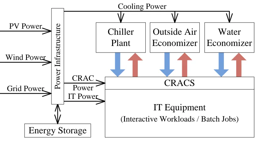
Figure 3.1 depicts an architectural overview of a sustainable data center. TheIT equipment includes servers, storage and networking switches that support applications and services hosted in the data center. The power infrastructure generates and delivers power for the IT equipment and cooling
1By “net-zero” we mean that the total energy usage over a fixed period is less than or equal to the local total
24 48 72 96 120 144 168 0
50 100 150
hour
renewable generation (kW)
solar wind
Figure 3.2: One week renewable generation
facility through a power micro grid that integrates grid power, local renewable generation such as photovoltaic (PV) and wind, and energy storage. The cooling infrastructure provides, delivers, and distributes the cooling resources to extract the heat from the IT equipment. In this example, the cooling capacity is delivered to the data center through the Computer Room Air Conditioning (CRAC) Units from the cooling micro grid that consists of air economizer, water economizer, and traditional chiller plant. We discuss these three key subsystems in detail in the following sections.
3.1.1
Power Infrastructure
Although renewable energy is in general more sustainable than grid power, the supply is often time varying in a manner that depends on the source of power, location of power generators, and the local weather conditions. Figure 3.2 shows the power generated from a 130kW PV installation for an HP data center and a nearby 100kW wind turbine in California, respectively. The PV generation shows regular variation while that from the wind is much less predictable. How to manage these supplies is a big challenge for application of renewable energy in a sustainable data center.
Despite the usage of renewable energy, data centers must still rely on non-renewable energy, including grid power and on-site energy storage, due to availability concerns. Grid power can be purchased at either a pre-defined fixed rate or an on-demand time-varying rate, and Figure 3.3 shows an example of time-varying electricity price over 24 hours. There might be an additional charge for the peak demand.
24
48
72
96
120
144
168
0
2
4
6
hour
electricity price (cents/kWh)
Figure 3.3: One week real-time electricity price
maximize the use of renewable energy while minimizing the use of storage.
3.1.2
Cooling Supply
Due to the ever-increasing power density of IT equipment in today’s data centers, a tremendous amount of electricity is used by the cooling infrastructure. According to [160], a significant amount of data center power goes to the cooling system (up to 1/3) including CRAC units, pumps, chiller plant, and cooling towers.
Lots of work has been done to improve the cooling efficiency through, e.g., smart facility design, real-time control and optimization [23, 183]. Traditional data centers use chillers to cool down the returned hot water from CRACs via mechanical refrigeration cycles since they can provide high cooling capacity continuously. However, compressors within the chillers consume a large amount of power [198, 145]. Recently, “chiller-less” cooling technologies have been adopted to remove or reduce the dependency on mechanical chillers. In the case with water-side economizers, the returned hot water is cooled down by components such as dry coolers or evaporative cooling towers. The cooling capacity may also be generated from cold water from seas or lakes. In the case of air economizers, cold outside air may be introduced after filtering and/or humidification/de-humidification to cool down the IT equipment directly while hot air is rejected into the environment.
0
24
48
72
96
120
144
168
0
0.2
0.4
0.6
0.8
1
hour
normalized CPU usage
Figure 3.4: One week interactive workload
usually complemented by more stable cooling resources such as chillers, which provides opportunities to optimize the cooling power usage by “shaping” IT demand according to cooling efficiencies.
3.1.3
IT Workload
There are many different workloads in a data center. Most of them fit into two classes: interac-tive, and non-interactive or batch. The interactive workloads such as Internet services or business transactional applications typically run 24x7 and process user requests, which have to be completed within a certain time (response time), usually within a second. Non-interactive batch jobs such as scientific applications, financial analysis, an