E20 8171 An Introduction to Linear Programming 1964 pdf

PREFACE

The purpose of this manual is to describe linear programming, to show what can be accomplished with it, and to prepare the reader to make intelli-gent use of a linear programming system on a com-puter. The presentation covers the entire scope of a linear programming application: problem formu-lation, computer operations, interpretation of results, and additional information that can be ob-tained through the use of a complete linear pro-gramming system for a computer. There is no attempt at mathematical rigor. Some of the mathe-matical techniques are presented briefly to indicate what is involved in the computer solution of a problem, but no mathematical background beyond high school algebra is assumed.

The glossary, however, is intended as a comprehensive list of technical terms associated with the solving of linear programming problems, rather than as a list of only those terms used in this manual. Furthermore, the definitions are written in a technical manner for the benefit of those readers who are studying linear programming on a deeper level than that of this introductory manual.

Copies of this and other

mM

mM

CONTENTS

Chapter 1: Concepts and Examples . 1 Distillate (heating oil) Blending. 26

Fuel Blending . 27

1.1: Example of Production Capacity 3.3: The Objective Function

Allocation . 2 and Constraints 27

1. 2: Example of Feed Blending 7 Objective Function

.

1. 3: Example of Investment Policy 9 Material-Balance Constraints 27

1. 4: Characteristics of a Linear Pipe-Still Constraints. 27

Programming Application. 13 Cat-Cracker Constraint 27

1. 5: Typical Linear Programming Fuel Oil-Blending Constraint. 27

Applications . 13 Heating Oil-Blending Constraints. 27

Refinery Scheduling . 13 Gasoline-Blending Constraints . 28

Paper Trimming. 14 3.4: Computer Input 29

Production Allocation. 14 3.5: The Solution. 29

The Optimum Policy 31

Chapter 2: Deriving Additional Information Changes in Allocation. 31

About a Solution . 15 Marginal Values. 31

Reduced Costs. 31

2.1: The Fundamental "Answer". 15 Sensitivity of Profit to

2.2: Changing Limits: Right-Hand Side Constraint Coefficients 33

Ranges and Marginal Values 16 Ranges of Optimum-Policy

2.3: Changing Objective Function Variables 33

Coefficients: Profit Ranges 18 Marginal Value Ranges 34

2.4: Tradeoffs: Rates of Substitution 19 3.6: Parametric Programming 34

2.5: Sensitivity to Technology . 20

2.6: Changing Several Things at Once: Chapter 4: The Simplex Method. 37

Parametric Programming 21

4.1: Geometrical Background 37

Chapter 3: A Larger Example - Oil Refinery 4.2: Algebraic Demonstration . 38

Scheduling 23 4.3: Summary. 40

3.1: The Physical Situation 23 Glossary. 41

3.2: The Operating Data . 25

Crude Supply 25 Bibliography. 63

Pipe-Still Operations . 25

Catalytic-Cracker Operation . 25 Index 64

CHAPTER 1: CONCEPTS AND EXAMPLES

Linear programming is a mathematical technique for determining the optimum allocation of resources (such as capital, raw materials, manpower, plant or other facilities) to obtain a particular objective (such as minimum cost or maximum profit) when there are alternative uses for the resources. Linear programming can also be used to analyze the eco-nomics of alternate availability of resources, alter-nate objectives, and so on.

A few brief examples may serve to indicate more concretely what can be achieved with linear pro-gramming:

1. A manufacturer makes a number of different products. Each product uses certain production re-sources, each of which is available in a limited amount. The manufacturer knows how much profit he makes from each product. How much of each product should he produce in order to make the maximum total profit?

2. A producer of livestock feed is required to provide certain amounts of various nutritional ele-ments in each sack of feed. He can obtain the vari-ous elements from different grains and supplements, and he knows the cost of each. What combination of grains and supplements should he use to meet the requirements at least cost?

3. The manager of an oil refinery is considering expanding the production of his plant by adding capacity at some point in the refining process. Of the many different processes involved in refining, which one should have its capacity increased so as to bring the greatest return on the capital expenditure? 4. Another manufacturer uses a large number of raw materials in the production of a line of products. The prices of his raw materials are subject to mar-ket fluctuations, and in some cases there are signif-icant price breaks for large orders. He has a choice of which raw materials to use. One of the materials he is not using at the moment might prof-itably be used if the price were lower. How much would the price have to drop before he could make a greater profit by using it instead of something else? 5. This same manufacturer is faced with another problem: one of the raw materials he is now using will be unavailable for a while because of a fire at the plant of one of his suppliers. Of the various al-ternative raw materials that he could use to replace it, which one will cause the least decrease in profit, considering that the introduction of a different mate-rial may charge the mixture of other matemate-rials he uses?

These examples emphasize the importance of linear programming. When a large number of in-terrelated choices exist, the best choice may be far from obvious. An intuitive solution may never un-cover the best approach, and there is seldom any guarantee that what appears to be a fairly good pol-icy is really the best.

Such problems often involve large amounts of money. A rational approach to the problems re-quires:

• A systematic way to represent the goal, or objective, of the system under stUdy.

• A systematic way to describe the limitations, or constraints, under which the system must oper-ate -- for instance, the limited amount of production resources in the first example given, and the mini-mum nutritional requirements in the second example.

• Some way to arrive at one policy out of the many possibilities, and to be sure that it is the best.

• Some way to explore the ramifications of changes in the stated problem (assuming, of course, that the best, or optimum, policy for the original objective and the original constraints has been de-termined).

In the third example, the refinery manager needed to know which capacity limitation could most profitably be relaxed. In the fourth example, the manufacturer needed to know the effect on his best policy of a change in the costs of materials. In the fifth example, the manufacturer needed to know how the nonavailability of one raw material would affect his profit and how to choose a new policy that would minimize this effect.

Most systems also contain at least some features to allow investigation of the effects of problem changes of various sorts. The user must also know enough about linear programming to interpret the results printed by the computer, and to decide what changes should be explored.

Ordinarily, the user does not need to know a great deal about how the computer finds the optimum policy or how it arrives at the effect of changes. He does, however, need to know the elements of these methods in order to formulate his problem most effectively and to interpret the results intel-ligently.

The three examples that follow are designed to serve four essential purposes for the user who wants to employ linear programming intelligently but who needs only a minimum knowledge of the methods of solution.

1. The examples introduce the characteristics of a problem that can be handled with linear pro-gramming. The technique is not the universal remedy for all management problems; it is impor-tant to know not only what can be done with linear programming, but also what cannot.

2. They introduce the idea of problem formula-tion. Linear programming requires that the prob-lem be stated in a specific manner (in terms of the objective and the constraints mentioned earlier). There is usually a certain amount of work involved in transforming a problem, as initially stated, into the form required for linear programming solution. 3. They indicate the method of computation of the optimum policy.

4. They reveal some of the information that can be derived from the solution to a linear program-ming problem, and they aid in interpreting the results.

Following these examples, Chapter 2 will discuss the types of changes in the problem that can be ex-plored. In Chapter 3 a representative problem is carried from formulation, through preparation of the computer input, interpretation of initial results, and the change information presented by the com-puter system. For the reader who wishes to know more about solution methods, Chapter 4 is an intro-duction to the simplex method, which is the basis of most linear programming systems on computers.

1. 1: EXAMPLE OF PRODUCTION CAPACITY

ALLOCATION

We can get an idea of the characteristics of a prob-lem that can be attacked effectively with linear

pro-illustration is realistic to the extent that business-men do face such problems, hut the problem pre-sented is much smaller than the linear programming problems that are handled with computer systems.

A small machine shop manufactures two models, standard and deluxe, of an unspecified product. Each standard model requires four hours of grinding and two hours of polishing; each deluxe model re-quires two hours of grinding and five hours of pol-ishing. The manufacturer has two grinders and three polishers; in his 40-hour week, therefore, he has 80 hours of grinding capacity and 120 hours of polishing capacity. He makes a profit of $3 on each standard model and $4 on each deluxe model. He can sell all he can make of both.

How should the manufacturer allocate his produc-tion capacity to standard and deluxe models; that is, how many of each model should he make in order to maximize his profit?

Let us begin by converting this problem state-ment into a mathematical form. Assign the symbol S to the number of standard models manufactured in a week, and the symbol D to the number of deluxe models. The profit from making S standard models and D deluxe models in a week, then, is

3S + 4D dollars

For instance, if five standard models (S = 5) and seven deluxe models (D

=

=

How can we express the restrictions on machine capacity? The manufacture of each standard uses four hours of grinding. Making S standard models therefore uses 4S hours. Similarly, the manufac-ture of D deluxe models uses 2D hours of grinding time, since the manufacture of one deluxe uses two hours. The total number of hours of grindingcapac-ity used in a week, therefore, is

4S + 2D

We said previously that 80 hours of grinding time was available, so we might be tempted to write

4S + 2D

=

80. "Must not exceed" can also be expressed as "must be less than or equal to", a more convenient expression. The mathematical symbol for "less than or equal to" is S. The correct formula for the restriction on grinding capacity would be

48 + 2D :5 80 hours

In the same manner, we arrive at the limitation on polisher capacity:

28 + 5D :5 120 hours

In view of the higher profit on the deluxe models, one might suggest that the optimum policy would be to make as many deluxe models as possible and for-get the standard models. Let us calculate how many deluxe models alone could be made, and record the corresponding profit for future reference. The limitation on grinder time provides that two times the number of deluxe models must not exceed 80, and the limitation on polisher time provides that five times the number of deluxe models must not exceed 120. Grinder capacity permits 40 deluxe models to be made; polisher capacity permits no more than 24 to be made. Therefore, 24 is the maximum number of deluxe models that could be made, even though this policy would consume only 48 hours of grinder time out of the 80 available. The profit with this policy is $96, since there is a $4 profit on each of the 24 deluxe models.

Let us now explore what the constraints (restric-tions, or limitations) on machine time mean in geo-metrical terms. We shall draw a graph on which the vertical axis represents 8 (the number of stand-ard models made in a week) and on which the hori-zontal axis represents D (the number of deluxe models). Now remember the first constraint that on grinder capacity 48 + 2D :5 80 hours. Let us con-sider only the "equal" part of the symbol for the moment, and rearrange the statement of the con-straint:

48 + 2D

=

so 2D

=

and D

=

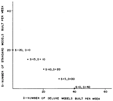
This equation lets us draw up a table of a few values of 8 and the corresponding values of D:

8

o

5

D

40

30

10 20

15

20

10

o

If we plot these points on a graph, the results would be those shown in Figure 1.

'"

I&J

~ 40

'"

...J

I&J

o o 2i ~ 20

«

o z

~ en

I&-o

en

5 =20, 0=0

.5=15,0= 10

• 5=10,0=20

• 5=5,0=30

5=0 0=40

20 40 60

0= NUMBER OF DELUXE MODELS BUILT PER WEEK

Figure 1. Five points that satisfy the equation 4S + 2D :::; 80

These five points lie on a line. We say that the equation 48 + 2D

=

Reviewing what the graph of our equation means, we have a straight line which "represents" the equa-tion in the sense that any point on the line corre-sponds to some specific combination of values of 8 and D, and these values satisfy the equation. With this meaning in mind, we can plot the equation of the constraint under consideration simply as a line, without identifying any of the specific points, as in

Figure 2.

a:: III Go !:i 3 ID (I) ..J III o i o

~ 2

z ;! (I)

...

0= NUMBER OF DELUXE MODELS BUILT PER WEEK

Figure 2. Graph of the equation 4S + 2D = 80

picture by any point on the line or below it. We can make this explicit by shading in the region that is covered by the inequality (see Figure 3).

a:: III Go !:i 3 ID (I) ..J III o o 2 o a:: c o z ;! (I)

...

0= NUMBER OF DELUXE MODELS BUILT PER WEEK

Figure 3. Graphical representation of the inequality 4S + 2D ~ 80.

Any point on the line or in the shaded region satisfies the inequality.

It is important to realize that any point on the line or below it still represents some specific com-bination of a value of S and a value of D; points be-low the line will be the "less than" part of the "less than or equal to" symbol.

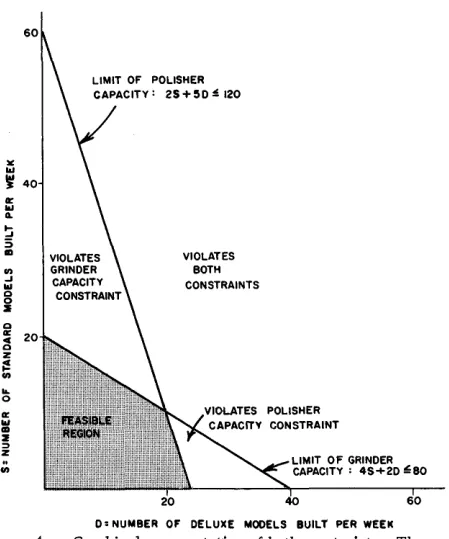
In Figure 4 we also plot the constraint on the polishing capacity (2S + 5D~ 120), but we now have shaded only the part of the graph that is ''below'' both lines. a:: III Go !:i 3 ID (I) ..J III o o ~ o a:: c o z ;! (I)

...

LIMIT OF GRINDER CAPACITY: 4S+2D ~80

0= NUMBER OF DELUXE MODELS BUILT PER WEEK

Figure 4. Graphical representation of both constraints. The small shaded region violates neither constraint and is called the feasible region.

In Figure 4 the shaded region reflects the effect of both constraints. The parts of the graph within the triangles violate one or the other of the con-straints; the part outside both lines violates both; the shaded region violates neither, and is therefore called feasible. This means tbat any point in the feasible region represents a combination of so many standard models and so many deluxe models, the combination being possible (feasible) with due re-gard for the amount of machine time available • From now on, we shall display only the feasible region on such graphs, since this area is all that really interests us.

the third example, "Investment Policy", and in Chapter 4 on the simplex method.

Here, we will see what can be done by graphical methods. We know that the profit for any particular point is 38 + 4D dollars. What would happen if we set this expression equal to some specific profit level, say $60? The answer is that we would have a linear equation, which we could plot as the broken line in figure 5. This line includes such points as 20 standard and zero deluxe models, 16 standard and three deluxe models, 12 standard and six deluxe models, eight standard and nine deluxe models, or zero standard and 15 deluxe models.

II: I&J Q. ~ :; m VI J I&J C o 2i c ~ 2

c z t! VI ... o \ \ \ \ \ \ \ \ \ \

GRINDER CAPACITY

e::--

POLISHER CAPACITY CONSTRAINT

40

0: NUMBER OF DELUXE MODELS BUILT PER WEEK

60

Figure 5. Graph of the constraints, the feasible region, and the profit line for $60: 3S + 4D 2 60

All points on this profit line are feasible; there is no violation of either machine capacity constraint anywhere on this line. Any point on this line thus represents a feasible policy, and all such points would return a $60 profit.

This policy, however, is not the best one. If, for instance, we try plotting the profit line 38+4D=$96, we find proof that there is a better policy (see Figure 6).

Not all points on this profit line are feasible. We cannot make 36 standard models and zero deluxe models, even though this point is on the line, be-cause there is not enough grinder capacity to permit it. Some points on the line are feasible, however; for instance, the combination of twelve standard models and 15 deluxe models violates neither con-straint and is therefore a feasible combination.

At $60, all points on the profit line were feasible; at $96 some points are feasible. The question that interests us now is the extent to which we can go and

~

I&J

~ 40

II: I&J Q. ~ :; m VI J I&J C 0 2i c II: C C z t! en

...

\ 60 \ \ \ \ \ \ \

RINDER CAPACITY CONSTRAINT

POLISHER CAPACITY CONSTRAINT

20 40

0: NUMBER OF DELUXE MODELS BUILT PER WEEK

Figure 6. The constraints and the $60 and $96 profit lines

still have at least one feasible point on the profit line. This point represents the optimum policy. To find it is the fundamental goal of linear program-ming' and we shall see that there are ways of working with algebra to arrive at it.

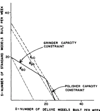
Staying with the graphical approach for now, we notice in Figure 6 that the two profit lines are paral-lel, an observation that can be proved

mathe-matically. Furthermore, all profit lines will be parallel for the problem as stated. This suggests a method of attack; look for the line parallel to the ones we have already drawn that goes as "far out" as possible but that still keeps one point in the feasible region. This will be the line that goes through the "corner" of the feasible region where the two constraint lines meet. It is shown in Figure 7. This is the profit line for $110, made from 10 standard models and 20 deluxe models.

It should be clear from Figure 7 that striving for any profit greater than $110 would involve a profit line with all points outside the feasible region. We have therefore established that $110 is the best profit that can be made under the original objective and constraints.

cr: 1&1 Q. !:i :5 III (I) -l 1&1 o o ~ o ~ 20

z i! (I) II. o cr: 1&1 III :I ::I Z \ \ \i'SO \ \ \ \ \ \ \

\

,

GRINDER CAPACITY CONSTRAINT

POLISHER CAPACITY CONSTRAINT

20 40

0: NUMBER OF DELUXE MODELS BUILT PER WEEK

Figure 7. The constraints and the $60, $96 and $110 profit lines

only by his unit profit on each product, but also by the constraints on his production capacity.

The problem of maximizing profit is representa-tive of a large class of problems that can be solved by linear programming. Such problems are charac-terized by the allocation of limited resources to products of different profitability.

It need not always happen, however, that the most profitable policy will require a combination of products. Suppose that the profit on each standard model was still $3, but that each deluxe model brought in $9 profit. When we search for the line with the greatest profit that still has at least one feasible point, we get the situation shown in Figure 8.

Here the profit line for the greatest profit that contains one feasible point still intersects the feasible region at one of its vertices (corners), but now it is a vertex formed of one of the constraint lines and one of the axes. This means that it is in-deed most profitable to make all deluxe models (24 in this instance) and zero standard models, even though this policy will leave 32 hours of grinder time unused.

It will be instructive to explore what the best policy would be if each standard model brought in $6 profit and each deluxe model brought in $3 profit. When we seek the greatest profit line that contains a feasible point, we get a profit line that coincides with one of the constraint lines, as in Figure 9.

The manufacturer has several choices of the best policy. He can make 20 standard and zero deluxe

cr: 1&1 Q. !:i :5 III (I) -l 1&1 o o ~ o

g

II. o cr:

..,

\

\ 3S -+ 90 : ~IS

\ /

D: NUMBER OF DELUXE MODELS BUILT PER WEEK

Figure 8. The constraints and the $216 profit line when the profit on a standard model is $3 and the profit on a deluxe model is $9

:II: 1&1 ~ 40 cr: 1&1 Q. !:i :5 III (I) -l 1&1 0 0 ~ 0 20 cr: C( 0 z i! (I) II. 0 cr: 1&1 III :I ::I Z (I)

~ ~GRINDER CAPACITY

~ CONSTRAINT

20

POLISHER CAPACITY CONSTRAINT

40

D: NUMBER OF DELUXE MODELS BUILT PER WEEK

Figure 9 The constraints and the best profit line when the profit on each standard model is $6 and the profit on each deluxe model is $3

standard and 20 deluxe models, since each combi-nation brings in the same profit of $120. Any of these combinations can be taken as the "best II policy;

they are all equally good. This type of solution occasionally appears in practical applications.

re-ordinary algebraic methods do permit negative numbers. This nonnegativity requirement becomes an integral part of the algebraic approach, but a person using a computer program based on such an algebraic method does not have to go to any extra effort because of the requirement.

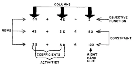
We are now in a position to state the original example in the standard form for a problem that can be handled with linear programming.

(1) Maximize

(2) Subject to

3S + 4D the objective function (profit)

4S + 2D::; 80 the problem 2S + 5D ::; 120 constraints

(3) And subject to S ~ 0, D ~ 0 the nonnegativity constraints

We shall refer frequently to the parts of the mathematical statement of a problem for linear programming solution. Figure 10 shows the termi-nology that will be used in this manuaL Note that the objective function has been set equal to Z as a convenience in later operations. Observe that a ~ refers to one constraint or to the objective function; one column refers to one activity or to the right-hand side. The values of the variables are called activity levels.

COLUMNS

J:

:J.

RowsE

3S ₊

FUNCTION

45 + 2 D ~

B O J

CONSTRAINTS 2S +

"

•

RIGHT HAND ACTIVITIES SlOE

Figure 10. The terminology used in describing the normal formulation of a linear programming problem

We shall see that the standard form of a problem suitable for linear programming is characteristic, although there are important variations: we often want to minimize a cost rather than maximize a

profit, and we often have constraints that state a "greater than or equal to" condition rather than a "less than or equal to" condition.

1.2: EXAMPLE OF FEED BLENDING

A poultry farmer needs to supplement the vitamins in the feed he buys. He is considering two products, each of which contains the four vitamins required, but in differing amounts. Naturally, he wants to meet (or exceed) the minimum vitamin requirements at least cost. Should he buy one product or the other, or should he mix the two? The facts are summarized in the table below.

Product 1 Product 2

Cost per ounce 3 cents 4 cents

Vitamin 1 per ounce 5 units 25 units

Vitamin 2 per ounce 25 units 10 units

Vitamin 3 per ounce 10 units 10 units

Vitamin 4 per ounce 35 units 20 units

The farmer must provide, per hundred pounds of feed, at least 50 units of vitamin 1; 100 units of vitamin 2; 60 units of vitamin 3; and 180 units of vitamin 4.

Let us state the problem in the standard form described near the end of the previous example.

The objective in this case is to minimize the cost of obtaining the required vitamins. Let PI repre-sent the number of ounces of product 1 purchased, and let P2 represent the number of ounces of product 2. Then the objective is to minimize

3P1 + 4P2

5P1 + 25P2 ~ 50

25P1 + 10P2 ~ 100

10P1 + 10P2 ~ 60

35P1 + 20P2 ~ 180

As always, we have the nonnegativity requirement on the variables, in this case the number of ounces of P1 and of P2 bought.

How does this problem compare with the earlier one? Before, we were trying to maximize profit; now we want to minimize cost. Before, we had two activities (manufacture of standard and deluxe models); now, we also have two activities (buying of two types of product). Before, there were two con-straints; now there are four. The nonnegativity requirement on each activity level never changes.

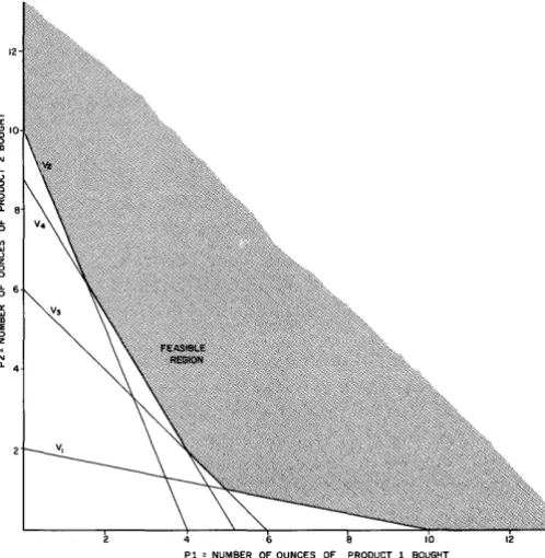
The situation is graphed in Figure 11.

Pi ' NUMBER OF OUNCES OF PRODUCT 1 BOUGHT

Figure 11. Graph of the constraints in the feed additive problem

The feasible region in this case is on the right-hand side of the lines, since the constraints are all "greater than or equal to "; there is no restriction on the amount by which the minimum can be ex-ceeded. The feasible region consists of all combi-nations of products that do not violate any of the constraints.

In Figure 12 we have shown only that part of each constraint line that is on the border of the feasible region, and we have plotted four total-cost lines.

12

10

10

Pt, NUMBER OF OUNCES OF PRODUCT t BOUGHT

Figure 12. Graph of the feed additive constraints and the total

cost lines for 12¢, 19¢, 30¢ and 4O¢

We see that the 129 line is not feasible anywhere and that the 409 line is feasible everywhere. Since the 199 line is the lowest-cost line that touches the feasible region, there is no possibility of getting the required vitamin content for less than 199. This corresponds to five ounces of PI and one ounce of P2, which minimizes the cost and still satisfies all four constraints.

One of the most valuable features of the methods used to solve general linear programming problems is that the methods guarantee that the optimum solution is the best. We have, of course, not proved this fact by the graphical demonstrations here, but the procedures used in linear programming guar-antee optimality.

requirements for the others in varying amounts; the cost would be 30¢. Ten ounces of P2 would satisfy exactly the requirement for the second vitamin and would cost 40¢.

Note that once again the optimum occurred at a vertex of the feasible region.

10 3: EXAMPLE OF INVESTMENT POLICY

Let us now turn to a rather different type of prob-lem. Because there are six activities, in this example, graphing (which is limited to two dimen-sions and therefore to two activities) cannot be employed. By deliberate choice, the optimum policy is rather obvious; the point of this example is to demonstrate an algebraic technique that will guarantee finding the optimum, even when the first guess at the optimum is far from accurate.

A man has $1,000 to invest. He has chosen to invest his money in some combination of municipal bonds, preferred stock, and common stock; for each, there are two candidates, making a total of six activities. The following table shows the yields and the symbols for the amount to be invested in each of the six possible activities.

Type: Bonds Preferred Common

Yield: 3% 3-1/2% 4% 4-1/2% 5% 5-1/2%

Symbol for Bl B2 PI P2 Cl C2

amount invested:

After consultation with his financial advisers, the investor decided upon the following restrictions on his investment policy: at least $400 must be in-vested in bonds; no more than $350 must be inin-vested in preferred stock; and no more than $350 must be invested in common stock. To make the problem statement concrete, his policy would permit placing $350 in the 5% common stock, or $350 in the 5-1/2% common stock, or any combination of the two that added to no more than $350.

Now we begin to convert the problem to the standard form of a linear programming problem statement. Converting the percentages to decimal fractions, the objective is to maximize

0.03 Bl + 0.035 B2 + 0.04 PI + 0.045 P2

+ O. 05 C 1 + O. 055 C 2

=

As noted near the end of section 1.1, we have given the objective function the symbol Z so that we can use it easily in writing equations.

The constraints this time are a mixture of equalities, "less than ", and "greater than" condi-tions. We begin with an ordinary equation, which states that the sum of the amounts invested must be exactly $1,000:

Bl + B2 + PI + P2 + Cl + C2

=

Next we have the "greater than or equal to" re-striction of at least $400 in either or both of the two types of bonds:

Bl + B2 ~ 400

Finally, we have two "less than or ,equal to" con-straints on the maximum that may be invested in preferred or common stocks:

PI + P2 ~ 350

Cl + C2 ~ 350

Because we are able to work more easily with equations than with inequalities, we therefore con-vert the three inequalities into equations by a simple technique.

Consider the second inequality, PI + P2 :s;; 350.

Let us introduce a slack variable, which we call S2, as follows:

PI + P2 + S2

=

What do "slack" and "variable" imply? Suppose that the optimum policy is to invest $250 in P2 and nothing in PI. Then the slack between the amount actually invested in the preferred stock and the maximum that is permitted would be $100. As we proceed through the calculations, the value of S2 may change before we arrive at the optimum; it is not fixed at any unchangeable value. In other words, it is truly a variable.

Note that with the introduction of a slack variable the result is equivalent to the original inequality. Like any other variable in a linear programming problem, slack variables are required to be zero or positive. Suppose that S2 were zero; then we would have PI + P2 = 350, which is the "equal to" part of

In other words, since 82 can vary, Pl + P2 can in-deed be less than or equal to $350. But the sum of Pl and P2 cannot be greater than $350, for that would require 82 to be negative, a condition which is not permitted.

In the case of the third inequality, introduction of the slack variable 83 leads to the equation:

C1 + C2 + 83 = 350

We suspect, of course, that the man will invest everything he can in this type; in other words, 83 will probably turn out to be zero, a value which is permitted.

In the case of the first inequality, which is of the "greater than or equal to" type, we must subtract the slack in order to represent the fact that he is permitted to invest more than $400 in the low-yield bonds--although he will not decide to do so. In other words, 81 will also eventually be zero.

Bl + B2 - 81

=

The minus sign here indicates subtraction, not that 81 is negative. As we have stated, the slack variables must be nonnegative, which means that they must be zero or positive. We are thus able to proceed with algebraic methods that depend on never having a negative variable--slack or otherwise.

Let us rewrite the four constraints as equations with slack variables where necessary. The equa-tions have been numbered for later reference.

(1) Bl + B2 + Pl + P2 + Cl + C2

=

(2) Bl + B2 -81 400

(3) Pl + P2 +82 350

(4) Cl + C2 +83

=

Here we have four equations in nine unknowns. There is no one single solution to such a system; there are many sets of positive values of the nine unknowns that will satisfy the equations. Our approach will be to pick five of the variables to be zero, and find values for the other four that satisfy the four equations. We shall then proceed in a sys-tematic way to see whether there are other ways to assign values that will improve the total yield.

The discussion of this process will be made somewhat easier if we first introduce some new

to the reader in any further study of linear program-ming methods. )

A solution with just as many variables permitted to be nonzero as there are equations, with all other variables being forced to be zero, is called a basic solution. The variables that are permitted to

"'i:ie

Can we find a basic feasible solution for this ex-ample? There are many ways to do so. Here is one: let B2

=

=

=

=

Having found any basic feasible solUtion, we seek to improve the basis; that is, we seek another basic feasible solution which is closely related to the first one but which gives a greater value to the objective function. If the basis can be improved still further, we repeat the process. Eventually, we shall find a basic feasible solution that cannot be improved, and we shall have arrived at the optimum solution.

Let us now use this process of improvement in the algebraic approach. First, express the ob-jective function entirely in terms of nonbasic variables; this will give a good clue as to where to seek improvement in the basis. This is easily enough done by finding expressions for the basic variables in terms of nonbasic ones, and by sub-stituting in the objective function.

We begin by solving the four equations (1) to (4) for the basic variables in terms of nonbasic vari-ables only. First we solve equation (2) for B2:

B2

=

Next, solve equation (3) for Pl:

PI

=

methods for doing this; in this example we shall take advantage of the characteristics of the system of equations to do it simply. First, subtract equation (2) from equation (1):

PI + P2 + Cl + C2 + SI = 600

Now subtract equation (3) from the above:

Cl + C2 + SI - S2

=

Now transfer everything except C2 to the right-hand side to get an expression for C2:

C2 = 250 - Cl - SI + S2

A similar scheme leads to an expression for S3. Subtract the original equations (2), (3) and (4) from equation (1) in turn, and rearrange:

S3

=

Now we can substitute these results into the ob-jective function:

0.03 Bl + 0.035 (400 + SI - Bl) + 0.04 (350 - P2 - S2) + 0.045 P2 + 0.05 Cl + 0.055 (250 - Cl - SI + S2)

=

By multiplying and rearranging, we get a trans-formed objective function:

$41. 75 - 00005 Bl + 0.005 P2 - 0.005 Cl - 0.02 SI + 0.015 S2 = Z

Observe that the objective function is now expressed entirely in terms of nonbasic variables. Where did the $41. 75 come from? That is the profit from the policy as it now stands, with the stated levels of the basic variables. We can demonstrate this another way, as in the following table.

Basic Activity Yield

Variable Level Rate Yield

B2 400 0.035 $14.00

PI 350 0.04 14.00

C2 250 0.055 13.75

S3 100 0.0 0.00

$41. 75

Thus the transformed objective function, now ex-pressed in terms of nonbasic (zero level) variables, states what would happen to the value of Z if any of the nonbasic variables were given nonzero values. This will be important in the next step of the optimization process.

In the preceding process, the problem con-straints were expressed in terms of equations by introducing slack variables into the three

in-equalities. We picked four of the nine variables and gave them values that satisfied the equations (and therefore satisfied the original inequalities as well). The four nonzero variables are then called basic variables and constitute a basic feasible solution. All other variables are zero. We next solved the four equations for the four basic variables and sub-stituted the results into the objective function.

(5)

(6)

By using these procedures, we have:

$41. 75 - 0.005 Bl + 0.005 P2 - 0.005 Cl - 0.02 SI + 0.015 S2

=

B2

=

(7) PI

=

(8) C2

=

(9) S3

=

It is important to remember that all variables now on the right-hand sides of these equations (6-9) and in the objective function (5) are nonbasic vari-ables and are therefore zero. Thus the profit from this choice of investments is $41.75.

Can this policy be improved? We know intui-tively that it can, but what tells us so mathe-matically? The answer is the existence of positive terms in the objective function. All variables in the objective function are now zero, but what would happen if we were to give some positive value to one of the variables multiplied by a positive coefficient (P2 or S2)? The profit, of course, would be in-creased.

should pick the "wrong" variable, in the sense that it is not the one that gives greatest improvement in the objective function, it means at worst some extra computation. We will eventually arrive at the optimum, no matter which variable is chosen.)

If S2 is brought into the basis, which variable will leave? This question is answered by searching for the equation that permits S2 to be given the largest possible value without forcing any other variable into the negative. Equation (6) provides no information: S2 does not appear there. Equation (7) shows that S2 could be 'as large as 350, which would force PI to zero and thus out of the basis; we keep this value in mind. Equation (8) does not limit the size of S2. Since it appears there with a plus sign, it could be given any positive value without forcing C2 to become negative. Equation (9) shows that S2 can be no larger than 100 without forcing S3 to become negative. This, then, is the equation that specifies the variable to leave the basis, since it is this equation that limits the value of the entering variable.

We now solve equation (9) for S2:

S2 = 100 + SI - S3

The variable S3 thus leaves the basis. Substi-tuting this result into equations (5) through (9) and rearranging, we get:

(10) $43.25 - 0.005 Bl + 0.005 P2 - 0.005 Cl - 0.005 SI - 0.015 S3 = Z

(11) B2 = 400 + SI - Bl

(12) P1

=

(13) C2 = 350 - Cl - S3

(14) S2

=

We see that removing S3 from the basis and re-placing it with S2 has improved the basis: the profit from the new policy is $1. 50 greater than before.

The basis can be improved still further, since there is still one variable with a positive coefficient in the objective function. Let us therefore bring this variable, P2, into the basis, and once again inspect our equations to see which variable should leave. Scanning down equations (11) through (14), we see that P2 appears only in equation (12), so P1 is the variable to leave the basis. Sol ving this

P2

=

As before, we substitute this result wherever P2 appears in equations (10) through (14), arriving at the following result:

(15) $44.50 - 0.005 B1 - 0.005 P1 - 0.005 C1 - 0.01 Sl - 0.01 S3 = Z

(16) B2

=

(17) P2 = 250 - PI - SI + S3

(18) C2 = 350 - Cl - S3

(19) S2 = 100 + Sl - S3

Now that all the coefficients in the objective function are negative, no further improvement could be made by making any of these nonbasic variables nonzero. The maximum possible profit is $44.50.

This reasoning is sound. The obvious course was to invest the minimum permissible ($400) in the 3-1/2% bonds, the maximum possible in the highest yield 5-1/2% common stock, and the rest in the higher yield of the two preferred stocks. Multi-plying $400 times 3-1/2%, plus $250 times 4-1/2%, plus $350 times 5-1/2% gives the same profit figure of $44.50; this should come as no surprise, but it is nevertheless reassuring to see that the algebra did arrive at the right answer.

More important, we have demonstrated that the algebraic approach does not depend on intuition. We have of course not proved that this method will always work; that belongs to mathematical texts. We have shown, for this example, that the algebraic approach resulted in the same answer as was obvious, and we further demonstrated that there could not possibly be any better policy. Assurance that there is nothing better is of great importance in practical applications, since, if we could see the best policy by looking at the problem, we would have no need for linear programming.

The method used in this example is essentially the simplex method, which is the basis for computer solutions of linear programming problems and which will be discussed in more detail in Chapter 4. For

1. 4: CHARACTERISTICS OF A LINEAR PRO-GRAMMING APPLICATION

Linear programming is a powerful tool of scientific management, but it is not a cure-all. It does have limitations in terms of the kinds of problems that can be solved and in the way the problems must be formulated. A listing of a problem's requirements will be both a necessary statement of the method's limitations and a good review of the basic ideas.

1. A problem for solution by linear program-ming methods must have a definite, identified, numerical goal. It is not adequate to say "Waste must be reduced", or "Somehow we have to improve customer service". The goal (objective function) has to be stated as the sum of a series of terms, each consisting of the product of the activity level and a constant multiplier which is the cost or profit per unit of that activity. The goal can only be to maximize the total profit or minimize the total cost, whichever is appropriate. ("Profit" and "cost" are generic terms, however. "Profit" includes total yield from a process, the total income including expenses, and so on; "cost" includes waste, amount of material used, total inventory, and so on. )

2. There must be separate and identifiable activities, and the level of each activity must be measurable in numerical terms. Examples of activities in this chapter have included the amount of a product to be manufactured, the amount of a vitamin supplement to be purchased, and the amount of money to be invested in a type of security. Iden-tification of the activities that affect the objective is often one of the major parts of formulating a linear programming applic a tion.

3. The activities must be interrelated. In the investment example of section 1.3, for instance, it would not be possible to set an objective that would maximize profit and at the same time minimize risk -- unless the investor could state in numerical terms how much more risky a high-yield security is than a low-yield one.

4. The restrictions must be identified and stated in numerical terms. It is not enough to say, "The bottleneck in this process is the stamping mill. " We must know just how many hours per day or week are available. If this availability can be altered by priority orders, or if it is necessary to include setup time, these factors must be included in the formulation. Failure to state all the constraints will generally lead to misleading results.

5. All activities must appear only in linear combinations, both in the constraints and in the

objective function. This means that the only way a constraint may ever be written is as a sum of products, each product consisting of a constant multiplier and a single variable. It is not permis-sible, for example, for two variables to be multi-plied together, for a variable to be squared, or for the square root of a variable to be taken. The same restrictions apply to the objective function.

Frequently, some of these limitations can be overcome. For instance, consider a petroleum pipeline application. The flow rate is not a linear function of pressure, because a small increase in pressure for high pressures would not produce the same increase in flow rate that the same small in-crease would produce at a lower pressure. In some cases of this kind it is possible to break the graph of flow versus pressure into a series of straight-line segments that approximate the true curve accurately enough. Therefore, even when a function is nonlinear (such as the above), it can often be represented satisfactorily in linear programming formulations. What is necessary is the skill to break the function into line segments or linear approximations. This technique, while not mathe-matically exact, is often useful and valid.

1. 5: TYPICAL LINEAR PROGRAMMING APPLICA TIONS

The examples presented in this chapter have neces-sarily been small and simple. Before going on to an exploration of the additional types of information that can be gained from linear programming

methods, let us describe some application areas of more realistic size and see what power linear pro-gramming provides in each of them.

Refinery Scheduling

An oil refinery involves, among other things, the blending of some combination of materials to pro-duce one or more different products. The goal can be either maximum profit per barrel, or maximum profit for the total operation (the two do not always lead to the same policy). The constraints describe the maximum supplies of available materials and several performance requirements on the different outputs, such as octane number and vapor pressure.

If, as usual, the blending process includes chemical operations to convert some of the available

A realistic problem would involve 400 to 600 activities and perhaps 200 constraints. With such a complex problem, we cannot accurately find an optimum unless linear programming methods are used. Naturally, oil refineries were in operation before linear programming came into wide use in the 1950s, and refinery managers have been making decisions on these matters for many years. The value of linear programming in such work lies in the large financial effect of small improvements. The manager's decision, reached by previous methods, may have been quite close to the optimum; but a few cents of profit per barrel is a great deal of money when multiplied by production rates in the tens of thousands of barrels per day. In fact, the petroleum industry is presently the largest user of linear pro-gramming. We shall explore a refinery scheduling problem in some detail in Chapter 3.

Paper Trimming

A common problem in the paper industry is deciding how to fill a group of orders so as to waste as little paper in trimming as possible. The manufacturer has roll stock in a variety of widths; his orders call for rolls differing in width and length. There may easily be hundreds of ways to cut the orders from the stock; each of these ways becomes one activity in a linear programming solution. The constraints are the widths of the stock rolls. (Length is not a constraint, assuming there is enough stock on hand to fill the orders.) The goal is to fill the orders with as little trim loss as possible.

Formulating this problem for linear programming is both easy and difficult. It is easy in the sense that unquestionably it can be done, and the mathe-matics involved is simple enough (although we will not go through it). It is difficult in the sense that

every possible way of cutting the rolls is an activity, and it can take a long time simply to write down all the constraints. This latter problem can be greatly reduced with the aid of the computer itself, letting the computer enumerate the possibilities. This is just one example of a fairly common technique: let

the computer help in preparing the input data, which is often voluminous.

Although the use of linear programming in the paper industry is not so extensive as in oil refining, the economic gains are significant. Trim losses can be held to approximately 1%, whereas without linear programming they are typically 5%. In an industry in which orders are expressed in tons, this can mean a great deal of money.

Production Allocation

In its general outline, the example in section 1.1 (standard and deluxe models) is quite typical--except, of course, for size. Even in that small problem, the optimum policy was not obvious from the problem statement, and naturally many problems are more complex than that one. There would ordi-narily be more products, more manufacturing

operations, and other types of restrictions. Ex-amples of the last-mentioned would be limits on men and machines independently, when not all machines are used full-time; limits on storage of parts or final products; and different scrap percentages for different activities.

Many other examples could be cited, since linear programming can be utilized in any situation that meets the general requirements stated in the pre-vious section, and in which there is sufficient potential economic payoff to offset the study and solution costs. Such applications have appeared in almost every segment of industry and the military, and the list is continually expanding.

CHAPTER 2: DERIVING ADDITIONAL

INFORMATION ABOUT A SOLUTION

In the previous chapter we learned something about the general characteristics of a problem that can be solved with linear programming; we saw some of the mathematical methods by which the optimum solution can be found; and we received an indication of the economic value of the technique. We also saw some ways in which it might be desirable to investigate a problem beyond the finding of one solution to the original problem statement.

One of the most powerful concepts of scientific management is the investigation of several possible alternatives, using a method such as linear pro-gramming, before making a final decision. For example, before deciding to add new capital equip-ment, we would like to study the return on capital in several possible places in the production process where new equipment could be added. Before de-ciding where to place new sales emphasis, we would like to know which mix of products offers the

largest profit potential. Before deciding where to put the most effort into improved contracts for the purchase of raw material, we would like to know which group of materials has the most influence on profit. Before deciding on an efficiency campaign, we would like to know which operations in the manu-facturing process are the best candidates for re-ducing overall costs, considering that some kinds of changes may suggest entirely new approaches to the process.

In other words, the one "answer" giving the single best policy for the problem as stated is often only the beginning of obtaining the information needed about the system under study. It is often equally important to know how that policy would be changed if the problem statement changed; would the profit increase or decrease, and would there be a different set of activities in the optimum policy?

This information can be gained by appropriately changing the mathematical statement of the prob-lem and then by rerunning it. This may take con-siderable computer time, which we would like to save if possible. Fortunately, methods have been developed to investigate the effects of changes with-out re-solving the whole problem. In this chapter we shall investigate some of these matters, con-centrating on the value of the information derived

rather than on the mathematical methods used. The mathematical techniques are not extremely diffi-cult, but it would take considerable effort to learn them. Furthermore, it is practical to gain the benefit of most of these techniques without a de-tailed understanding of the intricacies of the math-ematics.

2. 1: THE FUNDAMENTAL "ANSWER"

We begin any linear programming problem with a set of constraints that describe either limitations on resources or minimum requirements that must be satisfied. We also have an obj ective function that describes either the total profit to be obtained from the set of activities or the total cost of the set

of activities. The goal is to maximize or minimize (whichever is appropriate) the value of the objec-tive function, subject to the constraints.

The fundamental "answer" states the level of each activity for a maximum profit (or least cost) and gives the value of that maximum profit. This answer is found by some form of the simplex method.

From the mathematics used, we learn that there will never be more nonzero activities in an optimum policy than there are constraints; there may be fewer. This means, for instance, that in a prob-lem with two constraints and ten possible activities, at least eight of the possible activities will be at the zero level in the optimum policy. This would happen in Example 1 of section 1. 1 if there were other products besides standard and deluxe mod-els, but the only constraints were the grinder and polisher capacity. An optimum policy would never-theless contain only two products. If this proves to be meaningless in a practical problem, it indi-cates that constraints were omitted in the problem formulation. In Example 1, for instance, we care-fully stated the assumption that the manufacturer could sell all he could make of either the standard or deluxe model. In most realistic situations there would be limits on marketability that would require other constraints to be included in the formulation.

nonzero, but is permitted to be zero; a nonbasic variable must be zero.

Constraints are most commonly expressed as inequalities: "less than or equal to" or "greater than or equal to". An inequality is converted into an equation by the introduction of a slack variable. A slack variable, like all variables in a linear programming problem, must be zero or positive. Any constraint that is not "tight" in an optimum solution (that is, some capacity is not fully utilized) will result in aln optimum basis that includes a slack variable. The value of such a slack variable gives the amount by which the corresponding availability is underutilized, or by which a minimum specifi-cation is exceeded.

Let us restate the fundamental ideas in terms of an example, which will be used to illustrate all further developments in this chapter.

A manufacturer can make hex nuts, screws and bolts. Each pound of hex nuts requires four man-hours of labor and one hour of lathe time. Each pound of screws requires two man-hours of labor and one hour of grinder time. Each pound of bolts requires two man-hours of labor, one hour of lathe time, and three hours of grinder time. The manu-facturer makes $3 profit on each pound of hex nuts,

$2 on each pound of screws, and $2.50 on each pound of bolts; he can sell all he can make of each. How many pounds of each product should he make for maximum profit, and what is the profit?

The manufacturer produces other items, but he has decided that for the hex nuts, screws, and bolts he can allow twelve man-hours, two lathe-hours, and four grinder-hours each day.

Let H stand for the number of pounds of hex nuts, S for the pounds of screws, and B for the pounds of bolts. Then we can restate the problem in the usual mathematical form as:

Maximize 3H + 2S + 2.5B

&1bject to 4H + 2S + 2B ~ 12 man-hours

IH + IB ~ 2 lathe-hours

IS + 3B ~ 4 grinder-hours We have here three activities (production of hex nuts, screws and bolts) and thr(~ constraints (availability of man-hours, lathe-hours and grinder-hours).

The optimum policy can be found by application of the ideas presented in the previous chapter. Since we wish to concentrate now on results rather than on mathematical methods, we shall not go through the algebra, but shall simply state the result. The optimum policy is to produce one pound of hex nuts, four pounds of screws, and no bolts. One hour of lathe time will not be used. The maximum profit is $11.

The basis consists of the following variables: pounds of hex nuts, pounds of screws, and hours of unused lathe time. Thus there is a slack variable in the optimum basis.

A glance at the original problem statement will make this inclusion of a slack in the optimum basis seem plausible. Bolts were forced out because each pound of bolts requires three hours of grinder time, leaving little time for screws. If the manufacturer made a pound of bolts, grinder capacity would limit him to only one pound of screws instead of the optimum four pounds; and four pounds of screws clearly bring in more profit than one pound of bolts.

This justification of the plausibility of the answer is given to assure the reader that the answer is correct, not to suggest that such a justification is ordinarily possible. In most practical applications the problem is much too complex to see at a glance why the answer came out the way it did. If this were possible, there would probably be no need to use linear programming.

2.2: CHANGING LIMITS: RIGHT-HAND SIDE RANGES AND MARGINAL VALUES

Knowing that the optimum policy is to make one pound of hex nuts and four pounds of screws, and that this policy brings $11 profit, we will probably want to know the answers to questions such as the following. How would the profit be affected if

another man-hour of labor were made available? How would it be affected if two more man-hours were made available? How many man-hours could be added before the optimum policy would be to make some combination of products other than nuts and screws?

Mathematically, all these questions relate to changes in the values on the right-hand sides of constraints. The term for the effect on profit of a change in a right-hand side is marginal value. This is defined as the change in the value of the objective function caused by a unit change (a change of one in the value of the right-hand side of some constraint).

Computing the marginal values of the right-hand sides takes little extra effort, once the optimum has been found (although we shall not take the time to investigate the method). The values for the sample problem are:

Man-hours

Lathe- hours

Grinder- hours

$0.75

0.00

0.50

Taking man-hours first, one additional man-hour will raise the profit by 75~; two will raise it by

$1. 50; an added half hour will raise it by 37-1/2~.

It also means that removing man- hours will decrease the profit by 75 ¢ per man-hour removed. If the manufacturer has any other activity on which his profit on a man-hour is greater than 75¢, this marginal value would tell him immediately that he can make more money by shifting effort away from nuts and screws. It is precisely this type of infor-mation that is often of the most value in a linear programming application.

The zero marginal value of lathe- hours means that additional lathe-hours do not lead to any in-crease in profit. Since the manufacturer was not using all his lathe-hours initially, he could not make any additional profit by providing more capacity.

An additional hour of grinder time adds 50¢ to the profit. This may not seem reasonable, for how is it possible to increase grinder-hours without increasing man-hours, since a grinder presumably requires an operator? The answer is that it is not entirely reasonable; what the manufacturer might want to do is to investigate the effect of increaSing man-hours and grinder-hours Simultaneously. This is precisely the type of thing that is made possible by parametric linear programming, which will be discussed in section 2.6. For now, however, we must emphasize that marginal values here refer to changing one thing at a time, with all others held at

their original values. We cannot, for example, legitimately add the marginal values of man- hours and grinder-hours and say that the effect of adding one unit of each would be $1.25.

The marginal values nevertheless supply much useful information. Suppose that our goal were to provide a rational basis for deciding whether to buy a new lathe or a new grinder: the marginal values would indicate at once that for this part of the factory, at least, there would be no point at all in buying another lathe. Furthermore, the 50~ mar-ginal value of grinder time supplies information for computing the rate of return on a proposed capital expenditure for a new grinder.

The values given for the marginal values apply only as long as the optimum policy remains the making of hex nuts and screws and the leaving of some lathe-hours unused. Mathematically, we say that the marginal value s are valid only as long as the right-hand sides are not changed enough to re-quire a change of basis. (Recall that the optimum basis consists of hex nuts, screws, and unused lathe-hours.) If the number of man-hours is re-duced by one, we will make fewer hex nuts (as it happens), but we will still make some of them. We will still make screws, and there will still be some unused lathe-hours. In other words, a reduction of one man-hour does not change the basis, although it does change the value of one of the variables in the basis, and it does change the.total profit.

There is clearly going to be some limit on the amount by which the right-hand sides can be changed without requiring a change of basis. If we had only two man-hours, for instance, the optimum policy would be to make one pound of bolts, leaving unused lathe-hours and grinder-hours. The question is: What is the range of values for the right-hand sides, taken one at a time, that does not change the basiS, and over which range the stated marginal values are valid?

Information about the range of the right- hand sides can be provided with little extra computation once the optimum has been found. The results for this example are:

Lower Original Upper

Constraint Limit Value Limit

Man-hours 8 12 16

Lathe- hours 1 2 00 (infinity)

The table shows, for instance, that the number of man-hours available can range between eight and sixteen hours, with the other right-hand sides at their original values, and the optimum policy will still be to make hex nuts and screws, with some lathe- hours unused. The number of pounds and the profit will change, but the optimum policy will still be to make those two products. Furthermore, within this range, the effect on the profit of a change

in the number of man-hours will be to add 759 profit for each man-hour added. In other words, the marginal value given earlier is valid throughout this range.

What does it mean that although lathe-hours cannot be reduced below one without changing the basis, lathe- hours can be increased indefinitely without any such change? It. simply means that since we are not using all the lathe-hours available, our policy can never be affected by adding more.

What we are calling the marginal value is also called by other names, depending on the nature of the problem and on the writer: incremental cost, raw stock cost, break even price, simplex multi-plier, and shadow price. Shadow price is perhaps the most common alternative name; we prefer to avoid it because the same term is also sometimes applied to variation of the coefficients in the objec-tive function, leading to confusion as to the intended meaning.

2.3: CHANGING OBJECTIVE FUNCTION COEFFICIENTS: PROFIT RANGES

Just as we were interested in what would happen if the right-hand sides were changed, it is often

valuable to have similar information about the values in the objective function.

For any activity that is in the optimal basis, the concept of marginal value is the same as with the right-hand sides. What is the effect on the optimum profit when there is a unit change in the profit co-efficient for an activity? This information is generally not printed by the computer program, since it can be found by inspection of the objective function and from the levels of the optimum basic variables. For instance, if the profit on a pound of screws were $3 instead of $2, the profit would be increased by $4 since the optimum policy is to make four pounds of screws (and still one pound of hex nuts). For a nonbasic variable, changing the unit

profit has no effect on the total maximum profit. Since any nonbasic variable is zero, increasing its profit cannot raise the total profit. (That is, it cannot do so unless the unit profit change is great enough to cause a change of basis. We are assum-ing throughout this section that the basis doe s not change. )

Since the marginal values of the objective function are so easy to find, they are not printed; in fact, we do not ordinarily use the term "marginal value" in connection with the objective function. When we say "marginal value", it is understood that right-hand sides are intended.

Just as with the right-hand sides, however, there will be a limit on the range over which objective function variations do not cause a change in basis. Since the ranges of validity are not obvious from the objective function and the optimum basiS, they can be printed by the computer. They are called profit ranges (or cost ranges, where appropriate),

Lower Original Upper

Constraint Limit Value Limit

Hex Nuts $0.00 $3.00 $3.50

Screws 1. 83 2.00 00

Bolts -00 2.50 3.00

In the case of hex nuts, this means that as long as there is any profit in them, we shall make some of them; if, however, the profit for a pound of hex nuts were greater than $3.50, we would change the basis. For example, if the profit per pound of hex nuts were $4, the optimum policy would be 1. 5 pounds of hex nuts, 2.5 pounds of screws, and 0.5 pounds of bolts. There would be no unused capacity. Comparing with the optimum basis for the problem as stated, the activity of making bolts has entered the basis and lathe slack has left it.

The range on the making of screws indicates that

it was not profitable to make them anyway. If the profit for a pound of bolts rose above $3, howev