Thesis by
Gregory S. MacCabe
In Partial Fulfillment of the Requirements for the Degree of
Doctor of Philosophy
CALIFORNIA INSTITUTE OF TECHNOLOGY Pasadena, California
2019
© 2019
Gregory S. MacCabe ORCID: 0000-0003-2369-1580
graduate career possible: thank you for giving me the chance to learn from your brilliance in our field. There were numerous occasions when your insights, and discussions we had in your office or in the lab, revived my excitement for pushing the boundaries of our research together. I will always admire your determination and be imprinted with your optimism that good science is possible–even opportune–in the face of great technical difficulty. Thank you.
This thesis is a product of the accumulated experience, knowledge, and scientific tenacity which Oskar cultivates in his research Group at Caltech. I could not have performed the experiments presented here without relying heavily on the past developments and insights of the Group, and of Oskar – and I certainly did not do it alone. Thank you to all those who helped push this research as far as it’s gone, and who have helped me personally in its course. The environment of teamwork, collaboration, and shared enthusiasm for doing things right in the Painter Group is irreplaceable in my heart.
When I finished my undergraduate time at the University of North Carolina, I didn’t yet realize the extent to which my life would be enriched by traveling to California and studying physics in this historic place. I am deeply grateful to all the instructors and mentors I’ve been lucky enough to have through the years, both inside and outside Caltech. Jane Schelbe, Tom Clegg, Sean Washburn, Rich Superfine, Reyco Henning, John Engel, Tony Hotz, Rob Washeleski, Oskar Painter, numerous members of the physics and applied physics/materials science faculty at Caltech, and the friends and colleagues I’ve come to know along the way.
My greatest early influences in physics came from my dad, Stephen, and my older brother, Ken. I remember being about 12 years old when Ken first humored my curiosity about quantum oddities by telling me about the delayed-choice "quantum eraser." I think we have a shared respect for the fundamental mysteries of nature, but mine grew in large part from his. Some part of me has always found physics exciting because I knew that two of the people I admire most, Dad and Ken, shared in that excitement. Dad, thanks for always supporting my pursuit of science and math.
years. You brought me up to speed in the field and on projects for multiple years, and I’d hardly ever set foot in a cleanroom five years ago; now I only see right in yellow light. You gave me the instincts I needed to perform in this Group and you entrusted me with adding to your graduate work. I appreciate it. Seán Meenehan, I have an immense respect for your approach to problem-solving. Thanks for your guidance and discussions during my first couple years here.
To my closest collaborator and friend in the Group, Jared, what a journey it’s been. How many thousands of hours have we spent together poring over the optical setups and the data streams? How many thousands of texts, calls, and emails to keep such complex experiments running efficiently, or to get those fab recipes working just in time for a cooldown? There’s no replacing that, and there’s no overstating how rewarding it has been to work with you on these projects. You have a very bright future ahead, Mr. False-Trigger.
Many other past and present Group members have impacted me throughout my time here. Mahmoud, thanks for being a consistent friend through five years in the Group. I owe special thanks to Tim Blasius, Johannes Fink, Szilard Szöke, Roger Liu, Kejie Fang, Mohammad Mirhosseini, Su-Peng Yu, Andrew McClung, Hannes Pfeiffer, Paul Dieterle, Michael Fang, Andrew Keller, Neil Krueger, Anthony Ardizzi, Hengyun Zhou, Ewan Painter, Neil Sinclair, and others. Thanks to Michelle Rodriguez for your crucial support and conversations that helped buoy my mental state, Barry Baker for years of fixing things together, and Jonathan Gross for absolute reliability and being softball MVP. Thank you Guy DeRose, Melissa Melendes, Alex Wertheim, Nathan Lee, and the rest of the KNI staff.
To my mom, your love has enabled me to do what I do.
PUBLISHED CONTENT AND CONTRIBUTIONS
[1] G. S. MacCabe, H. Ren, J. Luo, J. D. Cohen, H. Zhou., A. Sipahigil, M. Mirhosseini, and O. J. Painter. “Phononic bandgap nano-acoustic cavity with ultralong phonon lifetime”. In:arXiv1.1901.04129 (2019).
G. S. M. Participated in fabricating the devices, planning and performing the experiments, analyzing the data, and preparing the manuscript.
[2] J.D. Cohen, S. M. Meenehan, G. S. MacCabe, S. Gröblacher, A. H. Safavi-Naeini, F. Marsili, M. D. Shaw, and O. J. Painter. “Phonon counting and intensity interferometry of a nanomechanical resonator”. In: Nature 520 (2015), pp. 522–525. doi:10.1038/nature14349.
G. S. M. Participated in fabricating the devices, performing the measure-ments, and analyzing the data.
[3] S. M. Meenehan, J.D. Cohen, G. S. MacCabe, F. Marsili, M. D. Shaw, and O. J. Painter. “Pulsed Excitation Dynamics of an Optomechanical Crystal Resonator near Its Quantum Ground State of Motion”. In:Physical Review X 5.041002 (2015). doi:10.1103/PhysRevX.5.041002.
Acknowledgements . . . iii
Abstract . . . v
Published Content and Contributions . . . vi
Table of Contents . . . vii
List of Illustrations . . . ix
List of Tables . . . xii
Chapter I: Prologue . . . 3
1.1 Extremely Long-Lived Acoustic Resonances . . . 6
1.2 Beginnings . . . 9
1.3 Dil Fridge Days . . . 10
Chapter II: Principles of Optomechanical Crystals . . . 12
2.1 Periodic Structures and Optomechanical Crystals . . . 13
2.2 The Optomechanical System Hamiltonian . . . 22
2.3 Dynamical Back-Action . . . 28
2.4 Heterodyne Detection . . . 34
Chapter III: Device Nanofabrication and Low-Temperature Optical Methods . 41 3.1 Nanofabrication Methods . . . 41
3.2 Dilution Refrigerator Optical Techniques . . . 55
3.3 Optical Characterization and Calibration at MilliKelvin Temperatures 60 Chapter IV: Phonon Counting and Phonon Intensity Interferometry . . . 66
4.1 Phonon Counting Theory . . . 67
4.2 Phonon Counting Sensitivity . . . 69
4.3 Phonon Intensity Interferometry . . . 71
Chapter V: Pulsed Excitation Dynamics of Optomechanical Crystals at Low Temperatures . . . 76
5.1 Pulsed Excitation Phonon-Counting Measurement Methods . . . 78
5.2 Calibration of the mechanical vacuum noise . . . 82
5.3 Thermal Ringdown and Bath Turn-On Dynamics . . . 84
5.4 Electromagnetically Induced Transparency at MilliKelvin Tempera-tures Using Single-Photon Detectors . . . 88
5.5 Mode Thermalization Measurements . . . 92
Chapter VI: Ultra-High-Quality Phonon Modes in Nanomechanical Resonators 96 6.1 Impact of Fabrication Imperfections on MechanicalQ-Factor . . . . 97
6.2 Impact of Acoustic Bandgap Shielding on MechanicalQ-Factor . . . 99
6.3 Properties of the Optical Heating Bath . . . 101
6.4 Coherent Excitation and Spectral Response of the Mechanical Mode . 111 6.5 Optomechanical Cooperativity . . . 123
Chapter VII: Phonon Decay and Decoherence at Low Temperature . . . 128
7.1 Mechanical Quality Factor: A Closer Look . . . 130
7.2 Thermoelastic Damping . . . 131
7.3 Phonon-Phonon Scattering Processes . . . 133
7.4 Strain Coupling to Two-Level Systems . . . 138
Chapter VIII: Epilogue: Future Directions for Optomechanical Crystals and Ultra-High-Quality Phonon Modes . . . 147
8.1 Quasi-2D Snowflake Optomechanical Crystals . . . 149
Bibliography . . . 159
Appendix A: Notation . . . 171
A.1 Fourier Transforms and Power Spectral Densities of Classical and Quantum Variables . . . 171
A.2 Operator Constructions . . . 172
A.3 Mechanical Power Spectral Density . . . 173
A.4 Scattering Matrix Elements . . . 174
Appendix B: Optical Cavity Coupled to a Thermal Bath . . . 175
Number Page 1.1 Summary of f Q-products for mechanical oscillators in cavity
op-tomechanics and related areas . . . 7
2.1 Canonical optomechanical system . . . 12
2.2 Periodicity in 1D photonic crystals . . . 17
2.3 Optical and acoustic modes of the nanobeam OMC . . . 18
2.4 Phononic crystal radiation shield image analysis and optimization . . 19
2.5 Band structure of the phononic crystal radiation shield "cross" pattern 20 2.6 Scattering picture for red- and blue-detuned driving . . . 28
2.7 Dynamical back-action damping and the optical spring effect . . . 32
2.8 Comparison of heterodyne and homodyne noise terms . . . 35
2.9 Single-port heterodyne detection illustration . . . 36
2.10 Balanced heterodyne detection illustration . . . 38
2.11 Balanced heterodyne output spectrum illustration . . . 40
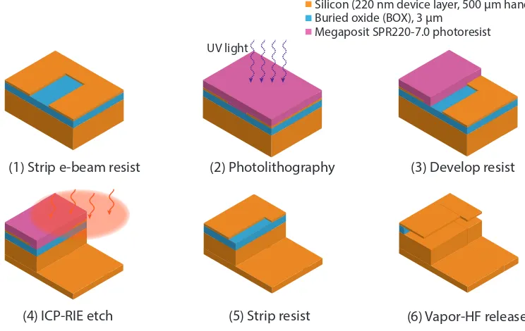
3.1 Silicon-on-insulator single-layer fabrication process flow . . . 43
3.2 End-fire device fabrication process flow . . . 48
3.3 End-fire device illustration . . . 49
3.4 Fabricated nanobeam device array . . . 50
3.5 Close view of the nanobeam OMC device cavity region . . . 51
3.6 End-fire processing used for integrated opto-electromechanical trans-ducers . . . 52
3.7 Lithography corrections and hole-fitting for nanobeam devices . . . . 54
3.8 Optical mode wavelength mapping at low temperature . . . 57
3.9 Side-coupling and tuning of the extrinsic optical quality factor . . . . 59
3.10 Single-photon detector calibration curve . . . 60
3.11 Characterization of the optical cavity using phase-sensitive detection 61 3.12 Room-temperature calibration of the vacuum optomechanical cou-pling rate in a nanobeam OMC . . . 64
4.1 Phonon counting sensitivity measured at room temperature . . . 70
4.2 Phonon lasing measurements at room temperature . . . 72
5.1 Schematic of the pulsed-excitation phonon counting technique . . . . 77
5.2 Pulsed-excitation phonon counting measurement setup . . . 79
5.3 Acousto-optic modulator optical pulse generation . . . 80
5.4 Transmission stability of the FFP filter stack . . . 81
5.5 Calibration of the mechanical vacuum noise for thermometry . . . 83
5.6 Phonon dynamics during the pulse . . . 85
5.7 Thermal ringdown of ultra-high-Qacoustic mode at low temperature 87 5.8 EIT mechanical spectroscopy using single-photon detectors at mil-liKelvin temperatures . . . 91
5.9 Base temperature occupancy measurement in a nanobeam . . . 93
5.10 Phonon counting sensitivity improvements . . . 95
6.1 Modeling of the breathing mode in the presence of fabrication disorder 98 6.2 Simulation of the impact of fabrication disorder on the mechanical Q-factor . . . 99
6.3 Measured mechanical Q-factor at low temperature for increasing acoustic shield depth . . . 100
6.4 Impact of the phonon bottleneck on the optical-absorption bath . . . 103
6.5 Techniques for extracting the optical-bath-induced damping rateγp. . 107
6.6 Pulsed measurements of the bath occupancy in a low-Qnanobeam . . 109
6.7 Properties of the optical-absorption heating bath in nanobeam OMCs at low temperature . . . 110
6.8 Mode occupancy during excitation and readout pulses for high-amplitude ringdown . . . 113
6.9 Coherently-excited high-phonon-number ringdown . . . 115
6.10 Phonon ringing-up dynamics . . . 118
6.11 Rapid measurement of the mechanical response and spectral diffusion 120 6.12 Time-averaged mechanical linewidth measurement using photon-counting at low pump power . . . 121
6.13 Temperature dependence of acoustic damping, frequency, and fre-quency jitter . . . 122
6.14 Cooperativity in quasi-1D OMCs at low temperature . . . 124
6.15 Low-temperature measurement of the self-oscillation threshold in a high-Qnanobeam . . . 127
7.1 Temperature dependence of the mechanical damping of ultra-high-Q acoustic modes . . . 130
phonon bath . . . 145 8.1 Entanglement distribution . . . 148 8.2 Quasi-2D OMC cavity modes based on the snowflake design . . . 150 8.3 Low-temperature characterization of a quasi-2D OMC device . . . . 151 8.4 Base temperature ringdown of a 2D OMC cavity with zero acoustic
shielding . . . 152 8.5 Base temperature thermalization of the 2D OMC cavity phonon mode 153 8.6 Properties of the optical heating bath in 2D OMCs at low temperature 154 8.7 Balanced heterodyne optical measurement setup . . . 155 8.8 Linewidth broadening in a 2D OMC due to bath-induced damping . . 156 8.9 Effective cooperativity measurement of a 2D OMC at milliKelvin
LIST OF TABLES
Number Page
0.1 Index of symbols and notation. . . 2
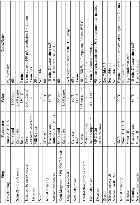
3.1 End-fire process flow details. . . 45
3.3 ICP-RIE optimized etch recipe parameters. . . 46
“And this I believe: that the free,
exploring mind of the individual
human is the most valuable thing
in the world. And this I would
fight for: the freedom of the mind
to take any direction it wishes,
undirected. And this I must fight
against: any idea, religion, or
government which limits or
destroys the individual. This is
what I am and what I am about.”
0 Permittivity of free space µ0 Permeability of free space kB Boltzmann’s constant Gth Thermal conductance
ωc Optical cavity resonance frequency ωL Laser drive frequency
ωLO Local oscillator frequency
∆ Laser-cavity detuning,∆=ωc−ωL ωm Mechanical resonance frequency
γ0 Intrinsic mechanical energy damping rate Qm Mechanical quality factor
meff Mechanical effective mass
κ Optical cavity energy decay rate,κ = κi+κe κi Intrinsic optical cavity decay rate
κe Extrinsic (coupling) optical cavity decay rate ˆ
a( ˆa†) Optical cavity mode bosonic annihilation (creation) operator ˆ
b( ˆb†) Mechanical mode bosonic annihilation (creation) operator
g0 Vacuum optomechanical coupling rate
nc Intracavity photon number,nc= haˆ †
ˆ ai
G Effective optomechanical coupling rate,G =g0 √
nc ¯
n Thermal phonon occupancy, ¯n= (e~ωm/kBT −1)−1 hni Average phonon occupancy
np Effective phonon occupancy of optically-induced heating bath nb Effective phonon occupancy of total effective mechanical bath γOM Optomechanical scattering rate,γOM =4g20nc/κ(∆=±ωm)
γp Mechanical heating bath-induced damping rate C0 Bare optomechanical cooperativity,C0= γOM/γ0
C Optomechanical cooperativity,C= γOM/(γ0+γp)
Ceff Effective (quantum) optomechanical cooperativity,Ceff=C/nb xzpf Mechanical zero-point fluctuation, xzpf=
Chapter 1
PROLOGUE
The fact that light exerts a force on matter has been known in some degree for centuries. Early scientific attention to this notion took the form of comments upon observations of apparently unrelated physical phenomena, the earliest of which is thought to be Kepler’s notes on the deflection of comet tails by solar irradiation in 1619 [1]. Over 250 years later, Sir William Crookes invented a hand-held radiometer device which rotates when irradiated with light—attracting a flurry of phenomenological theories aiming to explain its rotation as the result of an optical force [2]. In actuality the rotation of the Crookes radiometer is explained by thermodynamic effects [3], and the optical radiation pressure force as predicted by Maxwell’s full theory of classical electromagnetism [4] would not find direct experimental confirmation for a further two decades. This came in 1901 when Nichols and Hull developed a new radiometer, very similar to that of Crookes, but with appropriate sensitivity to detect Maxwell’s radiation pressure force to within 0.6% of its predicted magnitude [5].
In the decades that followed in the early 20th century, the quantum theory of light and its interactions with matter was rapidly maturing with herculean experimental studies of the photoelectric effect and blackbody radiation by Millikan, Einstein, Planck, and others. Einstein considered the effects of radiation pressure fluctuations on a movable mirror [6] in helping to develop the theory of blackbody radiation. In parallel with this, theoretical work by the Dirac and others aimed at understanding the interaction of light and matter at the level of single quanta—in particular to develop a theory of atomic spontaneous emission and level shifts in Hydrogen. In this era nearing the middle of the 20th century, the theoretical framework of quantum electrodynamics (QED) was resolving as the full quantum theory of light. The theoretical foundations provided by QED would underpin all later studies of the radiation pressure interaction at the quantum level.
laser light to cool ever larger mechanical objects attracted a great deal of scientific interest in the 1970s. Braginsky, Dykman, and others scrutinized the interaction of suspended mirrors and cavity light fields, largely in the context of developing ever better optical interferometers for position sensing, and identified regimes in which vibrations of a mirror may be either damped (cooled)oramplified (heated) by inter-actions with the light field (although these early experimental works were performed in the more experimentally accessible microwave frequency regime). A pioneer-ing experimental work by Dorsel [11] in 1983 found regimes of optical bi-stability arising from the radiation pressure in an optical cavity with a suspended movable end-mirror—begetting in theopticaldomain the field of cavity-optomechanics. In this field, the canonical physical picture is that of a Fabry-Perot cavity for which one of the end-mirrors is mechanically compliant and typically modeled as a harmonic oscillator linearly coupled to the circulating light field. In this picture, the motion of the end-mirror modulates either the phase or intensity of incident light, allowing readout of the position or momentum of the mechanical object with a sensitivity that may be limited only by quantum fluctuations in either the light field, the mirror position, or the detection electronics.
the SQL in optical sensing. In the following decade various proposals for circum-venting the SQL were made, usually relying either on injection of a squeezed optical vacuum to the interferometer—thereby suppressing quantum fluctuations in either the amplitude or phase quadrature—or by placing a Kerr medium in the optical path [13, 14]. Nevertheless, cavity-optomechanical systems (interferometers) have held great interest and demonstrated success as a platform for gravitational wave detection even in the presence of such an SQL.
In the last two decades, cavity-optomechanics has undergone a profound transfor-mation as its versatility in probing the physics of light-matter interaction has become both more apparent and more experimentally accessible with proliferation of optical materials fabrication and nanofabrication techniques. The use of a confined optical mode to cool macroscopic mirrors in 1999 [15] was in many ways the beginning of an ongoing effort to realize control of the acoustic and optical fields, as well as their energy exchange, at ever more delicate levels. Presently, cavity-optomechanical experiments are used for extremely broad classes of studies in the physics of light-matter interaction, quantum information science, gravitational wave detection, force and rotation sensing, gas sensing, and more. The physical principles that describe the light-matter interaction in a cavity-optomechanical system are germane over enormous ranges in size scale, from individual atoms trapped in focused light fields to kilogram-scale mirrors in the gravitational wave detectors of LIGO and VIRGO. The fact that the same system Hamiltonian and governing equations of motion can be used to analyze the dynamics and measurement imprecision over such disparate size scales gives cavity-optomechanics great relevance to human understanding of natural principles.
system known as an optomechanical crystal (OMC). These OMCs, which possess co-localized optical and acoustic modes with large coupling in a thin-film dielectric material, have previously been used to demonstrate sideband cooling of mesoscopic mechanical modes to the motional quantum ground state, optomechanically-induced transparency and slow-light, the generation of squeezed states of light, and more [16, 17, 18, 19, 20, 21]. The work presented here represents a concerted effort to optimize the technical performance of silicon OMCs with regard to manipulating phonon modes at the level of individual quanta, and generally to understand the physics governing their dynamical behavior at low temperature, in order that they may be useful in future hybrid quantum systems both for studying fundamental physics and for applications to the quantum control of matter using light.
1.1 Extremely Long-Lived Acoustic Resonances
A key figure of merit in cavity-optomechanical systems, and generally in oscillator systems which are coupled to a thermal environment, is the f Q-product of the cou-pled mechanical mode. The importance of the frequency and quality factor product can be understood by considering the number of coherent oscillations the resonator will experience before losing one quantum of energy to the thermal environment at temperatureT. The heating rate of an oscillator coupled to a thermal environment with occupancynth = (e~ωm
/kBT −
1)−1is [22]
Γ= γ~ωm
nth+ 1 2
, (1.1)
whereγ is the energy decay rate of the oscillator (Q = ωm/γ). Then the time for one quantum of energy ~ωm to be lost isτth = (γ(nth+1/2))
−1
, so the number of coherent oscillations is
ωmτth =
ωm
γ(nth+1/2)
≈ Q~ωm
kBT, (1.2)
of f Q = Qωm/2π kBT/~ ≈ 1013 is required for coherent quantum optome-chanics, whereas at typical dilution refrigerator base temperatures of 10 mK one requires a much more relaxed f Q 109 due to a greatly reduced thermal bath occupancy at low temperature. Figure 1.1 gives a summary of the f Qproducts re-alized for the mechanical element in various optomechanical and electromechanical systems representing the state of the art, with data adapted from Refs. [23, 24, 25]. The 5 GHz acoustic modes presented in this thesis obtain unprecedented energy coherence, reaching f Q = 2.6×10²⁰ and thermal decoherence times as large as τth =1.5 seconds.
Figure 1.1: Summary of f Q products achieved in cavity optomechanics and
related systems. Experiments in cavity optomechanics are represented by circles, with data adapted from Ref. [23], and the experiments presented in this work are represented by squares. Diamonds represent electromechanical/piezoelectric coupling to bulk acoustic modes, possessing some of the highest f Q products of any bulk material phonon modes prior to the work presented here [24, 25]. Item (1) is from Ref. [20], measured in a similar nanobeam OMC within the Painter Group prior to the work presented here, which is measured on an improved version of the same device platform. Items (2), (6), and (7) represent the work presented in this thesis [MacCabe:etal:2018, 26].
correspond to an optically-damped mechanical mode linewidth [19]. Moreover, at these frequencies the acoustic mode wavelength is close to the optical cavity mode wavelength (of order 1 µm), providing good mode overlap for generating optome-chanical coupling through radiation pressure. High-meoptome-chanical-frequency acoustic modes also minimize thermal occupation (thermal noise), and in our devices we have measured phonon occupancy as low as 10−3at an environmental temperature of 10 mK in a dilution refrigerator.
Perhaps most important, though, is the fact that our mechanical modes exist in the same frequency range as common superconducting qubits, suggesting a future for devices of this type in hybrid quantum systems which couple superconducting qubits to acoustic modes. With energy decay times greater than one second, these microwave acoustic modes present a potentially valuable resource in the context of superconducting quantum computing as energy storage elements. Ongoing ef-forts within the Painter Group are investigating the possibility of coupling similar vibrational modes in silicon to superconduting circuits in order to leverage their ultra-long lifetimes for storage of quantum information. The challenges in doing this are multitudinous, as one is then concerned with generating electromechanical coupling between the superconducting circuit and the localized acoustic mode with-out sacrificing the acoustic mode lifetime. This may be achieved with the use of a piezoelectric material (commonly aluminum nitride) which couples strain fields to electric fields. The technical challenges associated with introducing more com-plex materials systems into nanostructures harboring GHz cavity-acoustic modes are currently under investigation.
Going forward, the temptation to couple nonlinear quantum elements (e.g., qubits) to these high-Q acoustic modes is ever increasing. Various other research groups
with a footprint on-chip of only a few square microns owing to the slow speed of sound in silicon (or other future material systems) compared to that of microwaves in a superconducting circuit. Success in this endeavor may directly enable scalability of quantum-acoustodynamic devices simply because many hundreds or thousands of long-lived mechanical resonators can be placed in an on-chip area that would be occupied by only a handful of electrical microwave or SAW/BAW resonators.
1.2 Beginnings
With the demonstration of phonon intensity interferometry at room temperature in Ref. [31], the phonon-counting technique had matured. I became much more involved in performing measurements during this time period. Subsequent pulsed excitation measurements [26] of thenanobeamOMC device at milliKelvin temper-atures inside the dilution fridge required substantial build-up of the measurement setup, protocols, and data handling capabilities. Those measurements set the stage for a program of low-temperature OMC research that forms the bulk of my thesis work, and has been the most rewarding and enjoyable technical pursuit I’ve made thus far.
With the indication that our breathing mode mechanical lifetime could approach a millisecond, we were motivated to for the first time make a systematic study of the effectiveness of the acoustic bandgap radiation shielding which had been used in all previous cryogenic measurements of the nanobeam OMC [20, 21, 30, 32]. Previous works had made use of the shielding on the basis of numerical modeling, which indicated that substantial localization of the mechanical mode energy could be achieved with by clamping with the full-bandgap material to eliminate clamping losses. To prepare for this series of measurements, we spent time to re-optimize the fabrication process used to make OMC samples suitable for end-fire optical coupling in the dilution refrigerator (Chapter 3.2). This would allow us nearly 100% reliable fabrication of device arrays for future experiments, and enable us to couple to several dozens of devices on an individual chip sample during one cooldown cycle of the dil fridge.
than others. We observed a few devices with mechanicalQ-factors above 1 billion and, knowing that there was substantial room for improvement, embarked to generate a round of devices in which the acoustic bandgap was optimally centered around the mechanical resonance frequency. After refining the lithography feedback to achieve this, later measurements of the mechanical lifetime showed a much clearer trend of mechanical-Q with acoustic shield depth as well as extremely large saturated mechanical-Qfactors on the order of 40 billion for our 5 GHz mode.
PRINCIPLES OF OPTOMECHANICAL CRYSTALS
The fundamental feature of a cavity-optomechanical system is an optical cavity resonance in which the resonance frequency is sensitive to the motion of a me-chanical degree of freedom within the cavity. Consider for example the canonical optomechanical system in Figure 2.1, consisting of a Fabry-Perot cavity in which one end-mirror is mechanically compliant. Circulating photons inside the cavity impart an impulse to the mirror upon reflection, having magnitude 2~k per photon where k = 2π/λ is the wavenumber of a photon with wavelength λ. Given an average numberN of photons circulating inside the cavity of lengthL with round-trip time τ= 2L/c, one sees that the average radiation pressure force imparted on the mirror is FRP = 2N~ck/2L = N~ω/L. In a general sense then, maximizing the force per photon is equivalent to decreasing the length (or effective length, in the case of a photonic crystal cavity) Lof the cavity.
Figure 2.1: Canonical cavity-optomechanical system. The canonical optome-chanical system can be modeled by a Fabry-Perot cavity of effective length Leff in which one mirror is mechanically compliant. If the mirror has massmand resonant frequencyωm, its zero-point motion is given byxzpf=
p
~/(2mωm), and the position operator is given by ˆx = xzpf(bˆ
†+ ˆ
The Fabry-Perot cavity implementation of an optomechanical device is suitable for many macroscopic applications of optomechanics, such as in kilometer-scale grav-itational wave detectors. At the millimeter-to-centimeter scale, thin-film materials have instead been used in device architectures ranging from cantilever-mounted and torsional-oscillator mirrors for force sensing at high frequencies and near the quantum limit [33, 34, 35], to micro-fabricated membranes coupled to macroscopic optical cavities for microwave-to-optical transduction near the level of individual photons and generation of squeezed states of light [36, 37, 38, 39, 40], and in whis-pering gallery optical resonators [41]. At still smaller length scales, nanofabrication techniques allow replacement of the Fabry-Perot cavity architecture with analogous structures through patterning of dielectric and semiconductor materials down to feature sizes which are deeply sub-wavelength. The push to shorter length scales is partially driven by the desire to reduce the effective motional mass of the mechanical element, thereby increasing the acceleration imparted on the mechanics per reflected optical photon, as well as to achieve structures with large mechanical frequencies for the reasons outlined above. Each of these various implementations has advantages and disadvantages, but for the purpose of the work presented here, we will focus exclusively on photonic devices using near-IR light to couple to high-frequency me-chanical modes in structures known as optomeme-chanical crystals (OMCs), in which light can be confined to mode volumes near the theoretical minimum of (λ/2n)3. These OMCs are crystals in the sense that they are formed through periodic pattern-ing of semiconductor materials (here usually Si or SiNx) to support co-localized photonic and mechanical/acoustic vibrational modes. Silicon-based OMCs are able to reach mechanical frequencies in the microwave regime (∼ 1−10 GHz) owing to the large speed of sound in silicon (5−8 km/s) with optical resonances in the telecommunications bands from 1200−1600 nm reaching optical quality factors on the order of 106. Moreover, the extremely small photonic mode volume of these OMCs is accompanied by a correspondingly large electric field strength per photon, giving rise to the possibility for large optomechanical coupling rates through pho-toelastic coupling in which the refractive index change (effective cavity length) is sensitive to the electric field strength in the material.
2.1 Periodic Structures and Optomechanical Crystals
electro-photonic structure, the supported eigenmodes can be understood by investigating the form of solutions to Maxwell’s equations in a dielectric material:
∇ ·B=0 (2.1)
∇ ·D=4πρ (2.2)
∇ ×H= 1
c ∂D
∂t + 4π
c J (2.3)
∇ ×E=−1 c
∂B
∂t . (2.4)
We are interested in the solutions of these equations in dielectric materials in the absence of source termsρandJ, and which can be described as consisting of discrete regions of different dielectric constantsε= ε(r, ω). For now we will consider only lossless materials for which ε is real, and ignore any frequency dispersion of ε. In general numerical methods for solving for the modes of a structure, such as the finite-element method (FEM) solver packages in COMSOL Multiphysics [42], the full complex-valued anisotropic dielectric tensor ←→ε (r, ω) is used. The field amplitudes for general solutions of Maxwell’s equations will be linear combinations of the normal modes which are harmonic in time, of the form H(r,t) = H(r)eiωt and E(r,t) = E(r)eiωt. If we insert these temporal normal mode solutions into Maxwell’s equations, we obtain two curl equations of motion for the fields:
∇ ×E(r)+ iω
c H(r)=0 (2.5)
∇ ×H(r) − iω
c ε(r)E(r)= 0. (2.6) Eliminating the electric field from the coupled equations yields an electromagnetic master equation for the magnetic field:
∇ ×
1
ε(r)∇ ×H(r)
=
ω
c
2
Equation 2.7 has the familiar form of an eigenvalue problem in which the magnetic field profile in a given region parametrized by a dielectric constant ε(r) can be determined as a function of frequency [43]. The solutions to the master equation will be a set of normal modes. Additionally, because we have assumed the media in which the solutions exist is free of source terms, the field patterns must be transverse, further limiting the spatial forms of solutions to the master equation. In the specific case of photonic crystals, the material (described by ε(r)) is patterned periodically, such that in addition to finding electromagnetic field solutions which are harmonic in time, we will search for modes which are also harmonic in space. Bloch’s Theorem [44] tells us that the spatial normal modes will take the form of plane waves in a periodic medium,
H(r,t)=H0eik·reiωt, (2.8)
wherekis the wave-vector and and the transversality requirement amounts to requir-ing thatH0·k = 0. If we restrict ourselves to the case of a quasi-one-dimensional photonic crystal, in which periodicity of the material is realized in only one of the three spatial axes ( ˆx), the solutions have the form H(r,t) = H0(y,z)e
ikxxeiωt
The Nanobeam OMC
In the devices studied in this work, the principles of quasi-1D photonic crystals are used to generate optical defect cavities in a nanobeam photonic crystal. The beam consists of a suspended thin-film (220 nm) Si layer patterned into regions of alternatingeffectivedielectric constant by removing some of the dielectric material in elliptical holes, as shown in Figure 2.3. The resulting optical potential is then readily modulated by changing the relative filling fraction and lattice constant of a unit cell (see Figure 2.2). The optical cavity of the nanobeam consists of a series of "mirror" unit cells on either end of the nanobeam, in which a pseudo-bandgap at the defect mode resonance frequency exists due to the choice of lattice constant and filling fraction of the unit cells. The lattice constant is set by the wavelength of the defect mode in the material, here roughlya0 ∼ λ/nSi = 450 nm (nSi = 3.48 at 1550 nm). In the central defect region of the nanobeam, the lattice constant and elliptical hole geometry are modulated adiabatically along the length of the beam to form a symmetric optical potential [20], in which there exists a confined mode at approximatelyωc/2π =194 THz (free space wavelenth 1550 nm). Confinement in the transverse ( ˆy) and out-of-plane ( ˆz) directions are achieved by total internal reflection due to index contrast with the surrounding vacuum or air. However, there do exist radiation modes which are not confined to the z = 0 plane; these are classified by wave-numbers greater than the longitudinal wavenumber kx, or equivalently, ω > ckx. These radiation modes form a light cone, as shown in Figure 2.2b. Due to the presence of the light cone and nearby bands which can couple strongly to radiation modes, the photonic bandgap of the mirror region is really a pseudo-bandgap. Nevertheless, it is possible to tailor a central defect in such a way that the guided mode in the defect region experiences large reflectivity at the mirror portion of the beam. A final comment here regards the polarization of the defect mode. The modes of interest in thin-film OMCs are usually ˆz-symmetric with E-fields largely in the z-plane; thus, we classify them as "transverse-electric-like" (TE-like) modes. Details of the nanobeam optical cavity design are given in Ref. [20], and the geometry of the structure and the defect optical mode are shown in Figure 2.3.
periodic-x y
index n
a0
Field a
b
Figure 2.2: Periodicity in 1D photonic crystals. a, Alternating regions of high and low index with lattice constanta0can lead to constructive or destructive interference of propagating waves of wavelengthλ≈a0. An optical cavity can be constructed by combining two end-mirror regions with central defect region of different effective refractive index. b, A unit cell of the end-mirror portion of a nanobeam OMC, which is periodic in the ˆx direction, and the photonic band structure of the mirror portion [20]. Bands shown in red (blue) have odd (even) y-symmetry. Radiation modes exist forω > ckx. A pseudo-bandgap exists near ω/2π = 200 THz, in the vicinity of a defect mode of the central defect region of the nanobeam (dashed line).
ity of the nanobeam gives its structural acoustic normal modes a spatial periodicity as well. The central defect region of the nanobeam supports a so-calledbreathing acoustic resonance in the microwave frequency regime, here near 5 GHz. By tai-loring the mechanical properties of the defect region relative to the mirror regions at either end of the beam, the acoustic breathing mode is localized to the defect region. The mirror regions support a partial acoustic bandgap at the breathing mode frequency. Note that because the acoustic modes cannot radiate into the vacuum (unlike electromagnetic modes), they are confined to the plane of the nanobeam, and therefore the band-structure diagrams for the modes in the longitudinal axis of the nanobeam ( ˆx) do not contain light-cones of continuum modes.
Figure 2.3: Optical and acoustic modes of the nanobeam OMC. a, Scanning elec-tron microscope (SEM) image of a full nanobeam optomechanical crystal (OMC) device fabricated on silicon-on-insulator (SOI) with 7 periods of acoustic shielding. A central coupling waveguide allows for fiber-to-chip optical coupling as well as evanescent side-coupling to individual nanobeam OMC cavities. b, SEM image of an individual nanobeam OMC and the coupling waveguide, with enlarged il-lustration of an individual unit cell in the end-mirror portion of the nanobeam. c, Finite-element method (FEM) simulation of the transverse in-plane electric field magnitude|Ey|for the fundamental optical mode at ωc/2π = 194 THz (free-space wavelengthλc ≈1550 nm). d, FEM simulation of the displacement field magnitude of the "breathing" acoustic mode atωm/2π =5.0 GHz. Distortion of the mechanical mode profile is exaggerated for clarity.
Figure 2.4: Phononic crystal radiation shield image analysis and optimization.
a, SEM image of the clamping region of the nanobeam OMC, patterned with a phononic crystal "cross shield." b, Close view of several unit cells of the cross shield used for image fitting and analysis. c, SEM image of an individual unit cell of the cross-crystal acoustic shield. The dashed lines show fitted geometric parameters used in simulation, including cross height (hc = 503 nm), cross width (wc =169 nm), inner fillet radius (r1), and outer fillet radius (r2).
the structure supports a full acoustic bandgap≈ 3 GHz-wide around the breathing mode resonance frequency (gap-midgap ratio 0.6). The band structure of a realized cross shield is shown in Figure 2.5. The origin of the bandgap can be qualitatively understood as arising from the large difference in resonance frequencies of the square masses (high frequency) and narrow, floppy tethers by which they are connected (low frequency). In such a structure, the planar acoustic modes experience a full bandgap, and as the acoustic modes are also prohibited from radiating into the ˆz direction, the bandgap is fully three-dimensional.
0 1 2 3 4 5 6
Frequency (GHz)
Γ X M Γ
Figure 2.5: Band structure of the phononic crystal radiation shield "cross"
pattern. Acoustic band structure of the realized cross-crystal shield unit cell, with the full acoustic bandgap highlighted in pink. Solid (dotted) lines correspond to modes of even (odd) symmetry in the direction normal to the plane of the unit cell. The dashed red line indicates the nanobeam mechanical breathing-mode frequency atωm/2π = 5.0 GHz.
for calculation of band structure diagrams. Of particular importance in accurately modeling the acoustic bandgap structure is the inclusion of fillet curvature radii r1 and r2 of the concave and convex corners of the structure. This curvature arises from technical limitations of the lithography preventing the reliable fabrication of abrupt corners with curvature radii less than about 20 nm, and the fillet radii used in modeling substantially impact the frequencies of the upper and lower bandgap-edge modes. A lack of propagating modes in the acoustic shield region gives rise to an exponential decay of the acoustic field in that region as a function of position, which alternatively can be understood as a finite penetration depth of the acoustic mode in the bandgap material region. For sufficiently many periods of the acoustic shielding, the energy damping rate of the acoustic mode is not limited by radiation into the bulk (clamping losses), but becomes limited by other intrinsic material properties and defects, discussed in detail in Chapter 7.
Origins of Optomechanical Coupling
Rather than the real distance between the two end-mirros becoming modulated by reflected photons, theeffectivedielectric constant in the cavity region experienced by circulating photons is modulated by the mechanical motion. There are two main ways in which this can occur. First, mechanical motion will physically displace the boundaries of the dielectric structure, modifying the band structure and thus the frequency of the photonic mode. This change in boundary condition is referred to as a "moving boundary" effect. Second, the presence of a strain field in the dielectric can change the dielectric constant of that bulk material through the photoelastic effect.
The magnitude of the optomechanical coupling rate, defined as the rate of change of the optical resonance frequency as a function of mechanical displacementgOM = ∂ωc/∂αfor a generalized position coordinateα, can be decomposed into contribu-tions arising from the moving boundary effect and the photoelastic effect. This de-composition is useful in the design of OMCs, as the absolute and relative magnitudes of these contributions motivate the choice of which acoustic and electromagnetic modes should be used to tailor the device geometry. The total optomechanical cou-pling rate can be calculated by considering the effect of an infinitesimal mechanical displacement on the optical resonance frequency. The electromagnetic energy den-sity depends on the electric fieldEand dielectric constantε(r), and to first order in perturbation theory the change in energy can be calculated using the non-perturbed normal modes according to [20, 46]
gOM = ∂ωc Calculation of the moving boundary contribution to gOM can be performed by ignoring the strain-induced changes in ε to first order in α. In terms of the un-perturbed electric field mode profile and the mechanical mode profile q(r), the moving boundary contribution togOMis given by [47]
OM,ph
dielectric constant for the material [48]:
dε
Herepis the rank-four photoelastic tensor of the material andSis the mechanical mode strain tensor, with components
The resulting integral expression forgOM,phis
gOM,ph= 0 where the integral in the numerator is taken over the volume of the material. With expressions forgOM,bnd and gOM,ph, the total optomechanical coupling rate gOM =
gOM,bnd + gOM,ph can be calculated using the eigenmode solutions for the field
profilesEandqobtained by FEM simulations. The optomechanical coupling rate is conveniently expressed asg0= xzpfgOM, where xzpfis the zero-point mechanical amplitude and g0 therefore describes the optical cavity frequency shift due to the zero-point mechanical fluctuations (see Chapter 2.2). For the nanobeam OMC, typical contributions to the optomechanical coupling rate are numerically computed to be xzpfgOM,bnd/2π = −90 kHz and xzpfgOM,ph/2π = 860 kHz, giving g0/2π ≈ 770 kHz, in good agreement with the corresponding experimentally-determined coupling rates typically measured asg0/2π =700−900 kHz.
2.2 The Optomechanical System Hamiltonian
Let us more quantitatively investigate the origin of optomechanical coupling in the canonical cavity-optomechanical system. LetLeffbe the effective cavity length,meff be the effective mass of the movable mirror, k be the effective spring constant of the mirror. The mirror then has a mechanical resonance frequency ωm =
p
positive integer. Consider the fundamental optical mode at frequencyω0 =πc/Leff. As seen above, a single photon circulating in the cavity produces an average force FRP = ~ω0/Leff on the end-mirror. By Hooke’s Law this results in an average displacement ofx =~ω0/(Leffk), i.e., the cavity length isL+x. This shift in cavity length results in a shift of the optical resonance frequencies, which are now written to depend explicitly onx:
ωn−1(x) ≈
Assuming x Leff. The fundamental mode frequency is shifted by ∆ω0 = −(x/Leff)ω0= −~ω2
0/(kL 2 eff).
Modeling the system quantum mechanically we describe the optical and mechanical modes as quantum harmonic oscillators at frequencies ω0 and ωm respectively, where ˆa( ˆa†) is the bosonic annihilation (creation) operator for the optical mode and similarly ˆb( ˆb†) are the bosonic operators for the mechanical mode. The Hamiltonian of the quantum cavity-optomechanical system can then be written in terms of the self-energy terms of the modes as:
ˆ
H = ~ω0aˆ †
ˆ
a+~ωmbˆ†bˆ+Hˆint, (2.15)
where the term ˆHint describes the interaction of the optical and mechanical modes. We can find an expression for ˆHintby writingω0as an explicit function of the mirror’s displacement ˆx, following the simplified analysis above, so thatω0(xˆ)=ω0+
a. Now, the mechanical position operator ˆx =
xzpf(bˆ†+bˆ)is written in terms of the zero-point fluctuations xzpfof the mechanical
oscillator, xzpf =
p
h0|xˆ2|0i = p~/(2m
effωm). Then the interaction Hamiltonian is expressed as
fluctuations of the mechanical oscillator, we can write the full Hamiltonian reinforcing our intuition that increasing the optomechanical coupling is equivalent to decreasing the effective length of the cavity.
Generally we are interested in the dynamics of the optical and mechanical fields governed by Eqn. (2.19) under the influence of a strong coherent driving tone with frequency ωL. In this situation it is convenient to move into a reference frame rotating at the drive frequency–where the dynamics of the system operators on the optical timescale can be eliminated–in anticipation of later making a Rotating Wave Approximation. To do this, we define ˆA ≡ ~ωLaˆ
, and make the unitary transformation to the Hamiltonian:
ˆ
where the optical detuning is defined∆≡ ωc−ωL. The full Hamiltonian in general includes both additional driving and dissipation terms. We will append an explicit driving term ˆHdrive = ~(aˆ
†+ ˆ
a), but temporarily neglect dissipation. The constant here is proportional to the square root of the laser drive power, and is taken to be real. The system Hamiltonian is then
ˆ
H/~= ∆aˆ†aˆ+ωmbˆ†bˆ+g0aˆ†a(ˆ bˆ†+b)ˆ +(aˆ†+a).ˆ (2.22)
Linearization Approximation
due to the average radiation pressure force. It is then useful to re-formulate the Hamiltonian (and resulting dynamics) in terms of fluctuationsaboutthese coherent amplitudes. To this end we make the substitutions
ˆ
a −→αss+aˆ ˆ
b−→ βss+b,ˆ (2.23)
whereαss, βss are the coherent parts of the steady-state optical field and mechanical field, respectively. From here forward we drop the subscript "ss" for convenience. The substitution in Eqn. 2.23 is formally performed by applying a displacement to the Hamiltonian for each field:
Ignoring constant terms which have no effect on the dynamics, this is
ˆ
Taking α to be real, which amounts to using the phase of the coherent part of the optical field as a reference and therefore loses no generality,
ˆ
Now we observe that the effective driving terms for two fields, which are of the form (aˆ†+aˆ)and(bˆ†+bˆ)respectively, can be eliminated if we substitute the appropriate
Then
ˆ H/~=
∆− 2g0|α|2 ωm
ˆ
a†aˆ+ωmbˆ†bˆ+g0[α(aˆ†+aˆ)+aˆ†aˆ](bˆ†+bˆ). (2.28)
We see from this that the optical cavity obtains an effective frequency shift 2g0α2/ωm. This term is typically small, but can become large compared to the optical cavity linewidth κ at high intracavity photon number α2. It is simplest to re-define the optical detuning ∆to incorporate this shift. Further, we note that the interaction part of the Hamiltonian consists of terms which are products of two field operators and terms which are products of three field operators. The resulting Heisenberg equations of motion for these terms will respectively be linear and quadratic in the field operators; thus it will be useful to restrict the analysis to the terms which yield linear equations of motion. This linearization approximation is most valid in the limit of large α, where the nonlinear term ˆa†aˆ(bˆ†+ bˆ)is smaller by a factor of α than the dominant coupling terms. Under the linearization approximation, the full optomechanical system Hamiltonian can be written
ˆ
HOM/~= ∆aˆ†aˆ+ωmbˆ†bˆ+g0α(aˆ†+aˆ)(bˆ†+bˆ). (2.29)
We make a few observations about this optomechanical system Hamiltonian. First, the coupling strengthg0isparametrically enhancedby α=
√
N, the square root of
the intracavity photon number. This is a central result in linearized optomechanics, as it allows the effective coupling rate to be boosted and controlled by simply adjusting the input power to the system. We will follow a usual convention and define the enhanced effective couplingG≡ g0
√
N. Next, we note that the interaction
part of the Hamiltonian ˆHint = G(aˆ †+
ˆ
a)(bˆ†+ bˆ) in general contains four product
ˆ
It is straightforward to see then that depending on the choice of detuning ∆, some of the product terms will be rapidly-varying at twice the optical frequency, while some will be slowly-varying at approximately the timescale ofωm. We will make aRotating Wave Approximation(RWA) by neglecting the rapidly-varying terms in the Hamiltonian, which we will see correspond to energy non-conserving scattering processes within an intuitive picture of the optomechanical interaction.
Much like in the context of Raman scattering spectroscopy, in cavity optomechanics one is often interested in the Stokes and anti-Stokes motional optical sidebands generated by the acoustic mode through the optomechanical interaction. Thus the two non-resonant detuning parameters of greatest interest will be the higher-frequency (blue-detuned, Stokes-like) choice of∆= −ωm and the lower-frequency
(red-detuned, anti-Stokes-like) choice of∆= +ωm. Upon closer inspection of ˆHint above, we observe that for these choices of pump detuning we obtain
ˆ
Figure 2.6: The scattering picture for red- and blue-detuned driving. (a) Under the linearization approximation, the interaction Hamiltonian for a red-detuned (∆= +ωm) optical pump takes the form of a beam-splitter Hamiltonian. Pump photons are scattered into the cavity frequencyωc via absorption of a phonon, cooling and damping the mechanics. (b) For blue-detuned (∆ = −ωm) driving, the interaction takes the form of a two-mode squeezing Hamiltonian, whereby pump photons are scattered into the cavity frequency by emission of a phonon. This gives rise to correlated pairs of cavity photons and phonons, as well as amplification and anti-damping of the mechanics. For both∆= ±ωm, the scattered sideband atωc∓2ωmis suppressed by the reduced cavity susceptibility (according to the sideband resolution parameterκ/(2ωm)).
2.3 Dynamical Back-Action
The full optomechanical Hamiltonian (2.19) does not account for damping of the optical or mechanical mode annihilation operators, or noise inputs from the sur-rounding environment. In principle, the dynamics of the system will be governed in the Heisenberg picture by the equation of motion for any system operator ˆA, given by AÛˆ =−(i/~)[A,ˆ Hˆ]+∂Aˆ/∂t. However, in order to incorporate damping and noise inputs it is standard to use theinput-outputformalism of quantum optics describing cavities coupled to a noisy environment. The input-output formalism [49] allows the equations of motion for the optical and mechanical mode annihilation operators to be written:
rate to detection channels, and κi is the intrinsic loss rate to undetected channels (e.g., through scattering out of the cavity mode or absorption). The operator ˆain describes input to the cavity mode in the input-output formalism, and ˆain,idescribes noise input to the cavity mode via intrinsic loss channels (hereafter we will write ˆai
for notational convenience). Similarly, γi is the total mechanical energy damping rate, where ˆbinis a stochastic noise operator describing noise inputs to the mechanics which satisfies the bosonic commutation relation [bˆin(t),bˆ
† in(t
0)] = δ(t −
t0). The
input-output formalism yields a boundary condition for computing the output field at the extrinsic optical channel:
ˆ
aout =aˆin− √
κea.ˆ (2.33)
While the expressions 2.32 hold for general noise inputs, we usually assume that the mechanical mode is in thermal equilibrium at a temperatureTbhaving average phonon occupancynb =(e~
ω/kBTb−
1)−1. This gives rise to the noise correlators
hbˆ†
Using the Fourier Transform convention outlined in Appendix A, these can be written in the frequency domain as
hbˆ†
Similarly for the optical mode noise inputs we have the commutation relations [aˆin(t),aˆ†
in(t
0)] = δ(
t − t0) and [aˆin,i(t),aˆin,i(t0)] = δ(t − t0) for the extrinsic and intrinsic noise channels, respectively. The intrinsic noise is usually assumed to be thermal as well, but the corresponding noise occupancy of the optical bath is negligible at frequencies on the optical scale, effectively leading to ˆai as a vacuum noise input. Therefore, we use the correlators
haˆi†(t)aˆi(t0)i =0, (2.38)
haˆi(t)aˆi†(t)i =δ(t−t
0),
haˆi(ω)aˆ†i(ω0)i = δ(ω+ω0). (2.41)
In the preceding discussion we have explicitly separated the input optical noise into extrinsic (i.e., via a measurement channel) and intrinsic loss channels. We note that the noise on the extrinsic optical input ˆain is generally assumed to be vacuum noise unless otherwise stated, such that ˆain satisfies the same two-time correlators as ˆai.
In analogy with Section 2.2, we aim to simplify the analysis of system dynamics by making a linearization approximation by which we replace the system operators with operators describing fluctuations about some steady-state displacementsαand β. By solving Eqn. 2.32 in the steady-state, one finds the steady-state amplitudes in direct analogy with Eqn. 2.27 as
α=
where we have used nc = |α|2 is the intracavity photon number. Once again we choose the phase of α to be real without loss of generality going forward. As before we re-define the optical detuning to incorporate the static shiftg0(β
∗+ β) ≈ 2g02nc/ωm. Note that the steady-state drive amplitude ˆainis related to the generalized drive parameter in Eqn. 2.27 by ˆain =
√
κe. Now we may obtain the linearized Heisenberg-Langevin equations of motion by one of two equivalent methods: either by substitution of ˆa −→ α + aˆ, ˆb −→ β+ bˆ, ˆain −→ αin + aˆin into Eqn. 2.32 (ignoring terms beyond first order in the noise operators), or by using our linearized optomechanical Hamiltonian 2.29 along with the Heisenberg-picture prescription
Û ˆ
A=−(i/~)[Aˆ,Hˆ]+∂Aˆ/∂t. In either case we again include damping and noise terms according to the input-output formalism and arrive at the full linearized Heisenberg-Langevin equations of motion for the system annihilation operators:
where againG =g0αis the parametrically-enhanced optomechanical coupling rate. We can solve for the field amplitudes in the frequency domain by taking the Fourier Transform of Eqn. 2.43. In the frequency domain,
ˆ Inserting Eqn. 2.44 into Eqn. 2.45, we obtain an expression for the mechanical fluctuations entirely in terms of coherent and noise optical inputs:
ˆ
Defining the bare optical and mechanical susceptibilities, respectively χa(ω) ≡
(i(∆−ω)+κ/2)−1
lation operator in the frequency domain is
ˆ
The mechanical fluctuations are now found to be peaked around an optomechanically-shifted mechanical frequencyω0m, whereω
0
-2 -1 0 1 2 -4
-2
-2 -1 0 1 2
-1
Figure 2.7: Dynamical back-action damping and the optical spring effect. Plots of the normalized optical back-action modification to the mechanical damping rate (left) and to the mechanical frequency (right) as a function of detuning ∆, where we have chosen a ratioκ/ωm = 0.1 typical to the sideband-resolved systems in this work.
δωm(∆)=G2Im{χa(ω) − χa∗(−ω)} (2.51) =G2
Im
1
i(∆−ωm)+κ/2 −
1
−i(∆+ωm)+κ/2
, (2.52)
δγ(∆)=2G2
Re{χa(ω) − χa∗(−ω)} (2.53) =2G2Re
1
i(∆−ωm)+κ/2
− 1
−i(∆+ωm)+κ/2
. (2.54)
These dynamical back-action induced optical shifts to the mechanical frequency and damping rate are plotted schematically in Figure 2.7. In the second equality of the above expressions we have substituted ω −→ ωm since the mechanical response will be approximately constant over the bandwidth of the optical cavity, as γ κ holds in all systems considered in this work, and hence the mechanical response is only significant for frequencies|ω−ωm|. γ κ.
Sideband Resolved Systems
in the resolved sideband regime. In particular we consider the two detuning scenarios most relevant to experiment,∆= ±ωm, and find that we can write the optomechanical corrections to the mechanical frequency (the "optical spring") and damping rate as:
δωm(∆=±ωm)=±
The mechanical frequency shiftδωm ≈ (G2/2ωm)is typically small and unimportant in the studies presented here, but the optomechanical dampingδγis critically impor-tant. For convenience we will follow the convention to define the optomechanical damping term at∆=±ωm as
which is a strictly positive quantity, such that the total mechanical damping rate is given byγ = γi±γOM for∆=±ωm (red- or blue-detuning, respectively).
Generally we are interested in calculating and measuring the output optical field ˆ
aout in a cavity-optomechanical system using the boundary condition given by the
input-output formalism, and by this we are motivated to find simplified expressions for the optical fluctuation operator ˆa in terms of coherent and noise inputs from both the optics and mechanics. We consider the special case of red-detuning with ∆ = +ωm, where we find that we can write the mechanical fluctuation operator in Eqn. 2.50 in a simplified way:
ˆ
In the above expression we have defined a shifted mechanical susceptibility χ0b(ω)= (i(ω0m−ω)+γ/2)−1
and also chosen to neglect terms involving products of terms peaked near≈ +ωm and terms peaked near≈ −ωm, in particular χb0(ω) × χ
∗
a(−ω),
Substituting 2.59 into 2.44, and making use of the input-output boundary condition 2.33, we write an expression for the optical output fluctuations in terms of only optical inputs, optical noise, and mechanical noise fluctuation operators:
ˆ aout(ω)
∆=+ωm
≈ r(ω;+)aˆin(ω)+n(ω;+)aˆi(ω)+s(ω;+)bˆin(ω), (2.60)
wherer(ω;±),n(ω;±),s(ω;±)are optomechanical scattering matrix elements given explicitly in Appendix A.4. In a similar way we obtain for blue-detuning
ˆ aout(ω)
∆=−ωm
≈r(ω;−)aˆin(ω)+n(ω;−)aˆi(ω)+s(ω;−)bˆ†in(ω). (2.61)
2.4 Heterodyne Detection
Here we will give a brief review ofheterodyne detection, a method used in the work presented throughout this thesis to observe the mechanical noise power spectral density imprinted on the intracavity light field. Heterodyne detection (heterodyning) is a linear detection technique as it involves measuring a photocurrent proportional to the squared field amplitudes incident on a receiver. In heterodyne detection setups, a strong local oscillator (L.O.) amplifies a signal tone and mixes it into a frequency range which is convenient for detection. A special case of heterodyne detection–known as homodyne detection–in which the L.O. frequency is equal to the signal frequency, is also discussed for comparison to heterodyning. In homodyne detection, the L.O. frequency is matched to the signal frequency (often they are derived from the same laser source), allowing the relative phase of the L.O. to be controlled to perform detection of any desired quadrature of the signal. In general, the L.O. frequency may be chosen for a host of reasons, but is commonly used to either place the desired signal tone within a narrow radio-frequency detection bandwidth or to spectrally separate it from technical L.O. noise. These concepts are illustrated schematically in Figure 2.8.
Single-Port Heterodyne Detection
(a) Heterodyne (b) Homodyne
Field amplitude Field amplitude
Figure 2.8: Comparison of heterodyne and homodyne detection methods. a, In heterodyne detection, an offset frequency ∆ω between the L.O. and the signal frequency of interest (contained in the operator ˆa) is used to place the signal in a desired frequency band. This may be performed to mix a high-frequency signal to a lower frequency within the bandwidth of a receiver. In this work, a 5 GHz mechanical noise spectrum is routinely mixed to<100 MHz for detection on a high-gain RF photoreceiver. Noise on the local oscillator (indicated as ˆδb) is generically centered atωLO. Upon photodetection, a photocurrent is generated proportional to the squared field amplitude. Local oscillator noise is mixed to near DC while the signal spectrum is offset by∆ω. b, In homodyne detection, in whichωLO matches the signal frequency, L.O. noise is generically centered at the same frequency as the signal. Upon photodetection, the signal is mixed to to near DC. Because the L.O. and signal frequency are at the same frequency, the relative phase of the L.O. may be controlled in order to perform detection on any desired quadrature of the signal.
with one output ˆcmeasured on a photodetector producing a photocurrent ˆIc(t). For simplicity we will assume that the input and output ports of the beamsplitter are single-mode and single-polarization, allowing us to neglect any concerns of spatial mode-matching. In this context the input and output mode operators are bosonic mode continuum operators, in the Schrödinger picture, indexed by frequency (or in general, wave-vector), ˆa = aˆω. They satisfy the usual bosonic commutation relations,
[aˆω,aˆω†0]= δ(ω−ω
0),
(2.62)
Figure 2.9: A simple single-port heterodyne detection setup. An input signal ˆ
a and a strong local oscillator (L.O.) are incident upon a beam-splitter with trans-mission coefficient T and reflection R = 1-T. A beat note appears at the sum and difference frequency of the signal and local oscillator (frequency ωLO). At the output of the beam-splitter, one port is used to generate a photocurrent (here, mode
ˆ
c), which will consist of the beat-note terms as well as a DC term and terms arising from noise on the LO.
ˆ a(t)=
∫ ∞
−∞ dω 2πe
−iωt
ˆ
aω, (2.63)
as having units of square root of flux Hz1/2 ∼ pphotons/s. These ˆa(t) should not be confused with the Heisenberg picture operators used in the quantum Heisenberg-Langevin formalism of the previous section, but instead are simply constructs written in terms of the Schrödinger-picture continuum operators. It is straightforward to show that the Heisenberg operator ˆa(ω) is related to the continuum operator by
ˆ
a(ω)= 2πaˆω(0).
Now, a main objective of heterodyne detection is to amplify a weak signal by a strong coherent local oscillator (L.O.) amplitude, and hence we will assume the local oscillator amplitude may be written as
ˆ
b(t) βe−iωLOt+δb(tˆ ), (2.64) whereβ ∈Cis a large coherent field amplitude, equal to the square root of the average L.O. photon flux, and ˆδb(t)contains all the L.O. noise, including both vacuum noise and technical noise. If we assume an ideal detection quantum efficiencyηQE= 1 and a beam-splitter transmission coefficientT = 1− R, we may write the (normalized) photocurrent generated by the output ˆcas
ˆ
Ic(t)=Taˆ†aˆ+Rbˆ†bˆ+i √
the relevant fields relative to the L.O. For example, ˆa(t) = a˜ˆ(t)e−iωLOt. Then the
Referring the quadrature operator definitions as introduced in Appendix A.2, we can write this in a simpler form:
ˆ
We will refer to this result later, using the fact that the photocurrent consists of the position quadrature of the signal field amplified linearly by the local oscillator amplitude. The measured photocurrent consists of a DC term, quadrature of the signal mode ˆa, and a quadrature of the L.O. noise operator ˆδb. In this case, both the signal and noise terms are linearly amplified by the L.O. strength β. A more powerful measurement technique might be desired to eliminate such noise terms on the output photocurrent.
Balanced Heterodyne Detection
The photocurrent obtained in Equation 2.67 contains both a large D.C. offset term and an amplified local oscillator noise term proportional toβxˆδb,φLO. Thesecommon modenoise terms can in principle be eliminated with the use of a more sophisticated technique known as balanced heterodyne (homodyne), in which the previously discarded output port of the beam-splitter is used as a resource for noise reduction by measuring the difference in photocurrents at the two beam splitter output ports.
The generic balanced heterodyne setup is sketched in Figure 2.10, in which the output field ˆaoutfrom a cavity-optomechanical system is sent to to an idealized beam-splitter along with a strong L.O. tone. The difference photocurrent ˆI−(t) between the two output port photocurrents is measured. In direct analogy to Equation 2.65 it is straightforward to see that the difference photocurrent may be written
-Figure 2.10: Balanced heterodyne detection of a cavity-optomechanical
sys-tem output field. A single-mode, single-polarization field ˆain is input to a cavity-optomechanical system. The output field ˆaout is sent to a balanced het-erodyne/homodyne detection setup, here modeled as an ideal 50/50 beam-splitter and two photodetectors. A local oscillator of frequency ωLO is mixed with the signal ˆaout on the beam-splitter. Measuring the difference photocurrent from the two photodetectors allows common-mode noise of the local oscillator to be rejected (to some common-mode rejection ratio CMRR, typically 35−60 dB).
detection, here we do not have any noise terms going likeβδˆb, amplified by the local oscillator. In our Heisenberg-Langevin formalism using the input-output operators as expressed in Equations 2.60 and 2.61, this can then be written in the frequency domain as
Let us consider as an illustrative example the case of a sideband-resolved system un-der red-detuned (∆= +ωm) driving as measured on a balanced heterodyne detection setup. Then Equation 2.60 gives the output field in terms of reflection coefficients and fluctuation operators, and we may directly write an expression for the power spectral density of the difference photocurrent using Equation A.8: