A New Approach to Word Sense Disambiguation

(1)

A N e w A p p r o a c h to W o r d S e n s e D i s a m b i g u a t i o n

Rebecca Bruce and Janyce Wiebe

The Computing Research Lab

New Mexico State University

Las Cruces, NM 88003

A B S T R A C T

This paper presents and evaluates models created according to a schema t h a t provides a description of the joint distribution of the values of sense tags and contextual features t h a t is potentially applicable to a wide range of content words. The models are evaluated through a series of experiments, the results of which suggest t h a t the schema is particularly well suited to nouns but t h a t it is also applicable to words in other syntactic categories.

1. I N T R O D U C T I O N

Assigning sense tags to the words in a t e x t can be viewed as a classification problem. A probabilistic classifier assigns to each word the tag t h a t has the highest estimated probability of having occurred in the given context. Designing a probabilistic classifier for word-sense disambiguation includes two main sub-tasks: specifying an a p p r o p r i a t e model and estimating the p a r a m e t e r s of t h a t model. T h e former in- volves selecting informative contextual features (such as collocations) and describing the joint distribution of the values of these features and the sense tags of the word to be classi- fied. The p a r a m e t e r s of a model are the characteristics of the entire population t h a t are cohsidered in the model. Practical applications require the use of estimates of the parameters. Such estimates are based on functions of a d a t a sample (i.e., statistics) rather than the complete population. To make the estimation of p a r a m e t e r s feasible, a model with a simplified form is created by limiting the number of contextual features considered and by expressing the joint distribution of features and sense tags in terms of only the most i m p o r t a n t systematic interactions among variables.

To date, much of the work in statistical NLP has focused on p a r a m e t e r estimation ([11], [13], [12], [4]). Of the research di- rected toward identifying the o p t i m u m form of model, most has been concerned with the selection of individually informative features ([2], [5]), with relatively little attention di- rected toward the identification of an o p t i m u m approximation to the joint distribution of the values of the contextual features and object classes. Most previous efforts to formu- late a probabilistic classifier for word-sense disambiguation did not a t t e m p t to systematically identify the interdependencies among contextual features t h a t can be used to clas- sify the meaning of an ambiguous word. Many researchers have performed disambiguation on the basis of only a single feature ([61, [15], [2]), while others who do consider multiple contextual features assume t h a t all contextual features are either conditionally independent given the sense of the word (Is], [14]) o r fuRRy independent ([10], [16]).

J In earlier work, we describe a m e t h o d for identifying an up- propriate model for use in disambiguating a word given a set of contextual features. We chose a particular set of contextual features and, using this m e t h o d , identified a model incorporating these features for use in disambiguating the noun interest. These features, which are assigned a u t o m a t i - cally, are of three types: morphological, collocation-specific, and class-based, with part-of-speech (POS) categories serving as the word classes (see [3] for how the features were chosen). The results of using the model to disambiguate the noun in- terest were encouraging. We suspect t h a t the model provides a description of the distribution of sense tags and contextual features t h a t is applicable to a wide range of content words. This paper provides suggestive evidence supporting this, by testing its applicability to the disambiguation of sev- eral words. Specifically, for each word to be disambiguated, we created a model according to a schema, where t h a t schema is a generalization of the model created for interest. We eval- uate the performance of probabilistic word-sense classifiers t h a t utilize m a x i m u m likelihood estimates for the parameters of models created for the following lexical items: the noun senses of bill and concern, the verb senses of close and help, and the adjective senses of common. We also identify upper and lower bounds for the performance of any probabilistic classifier utilizing the same set of contextual features, as well as compare, for each word, the performance of' (1) a classifier using a model created according to the schema for t h a t word, with (2) the performance of a classifier t h a t uses a model selected, per the procedure to be described in section 2, as the best model for t h a t word given the same set of contextual features.

Section 2 of this paper describes the m e t h o d used for selecting the form of a probabilistic model given sense tags and a set of contextual features. In section 3, the model schema is presented and, in section 4, the experiments using models created according to the schema are described. Section 5 discusses the results of the experiments and section 6 discusses future work.

2. M O D E L S E L E C T I O N

In this section, we address the problem of finding the model t h a t generates the best approximation to a given discrete probability distribution, as selected from among the class of decomposable models. Decomposable models are a subclass of log-linear models and can be used to characterize and s t u d y the structure of data. T h e y are m e m b e r s of the class of gen- eralized linear models and can be viewed as analogous to analysis of variance (ANOVA) models ([1]. T h e log-linear

(2)

model expresses the population mean as the sum of the contributions of the "effects" of the variables and the interactions between variables; it is the logarithm of the mean t h a t is linear in these effects.

Under certain sampling plans (see [1] for details), d a t a con- sisting of the observed values of a number of contextual features and the corresponding sense tags of an ambiguous word can be described by a multinomial distribution in which each distinct combination of the values of the contextual features and the sense tag identifies a unique category in t h a t distribution. The theory of log-linear models specifies the su.~cient statistics for estimating the effects of each variable and of each interaction among variables on the mean. T h e statistics are the highest-order sample marginal distributions con- raining only inter-dependent variables. Within the class of decomposable models, the maximum likelihood estimate for the mean of a category reduces to the product of the sample relative frequencies (counts) defined in the sufficient statistics divided by the sample relative frequencies defined in the marginals composed of the common elements in the sufficient statistics. As such, decomposable models are models t h a t can be expressed as a product of marginal distributions, where each marginal consists of certain inter-dependent variables.

The degree to which the d a t a is approximated by a model is called the fit of the model. In this work, the likelihood ratio statistic, G 2, is used as the measure of the goodness of fit of a model. It is distributed asymptotically as X 2 with degrees of freedom corresponding to the number of interactions ( a n d / o r variables) omitted from (unconstrained in) the model. Ac- cessing the fit of a model in terms of the significance of its G 2 statistic gives preference to models with the fewest number of interdependencies, thereby assuring the selection of a model specifying only the most systematic variable interactions.

Within the framework described above, the process of model selection becomes one of hypothesis testing, where each pattern of dependencies among variables expressible in terms of a decomposable model is postulated as a hypothetical model and its fit to the d a t a is evaluated. The "best fitting" model, in the sense t h a t the significance according to the reference X 2 value is largest, is then selected. The exhaustive search of decomposable models was conducted as described in [9].

Approximating the joint distribution of all variables with a model containing only the most i m p o r t a n t systematic interactions among variables limits the number of p a r a m e t e r s to be estimated, supports computational efficiency, and provides an understanding of the data. The biggest limitation as- sociated with this m e t h o d is the need for large amounts of sense-tagged data. Inconveniently, the validity of the results obtained using this approach are compromised when it is applied to sparse data.

3 . T H E M O D E L

Using the method presented in the previous section, a probabilistic model was developed for disambiguating the noun senses of interest utilizing automatically identifiable contextual features t h a t were considered to be intuitively applicable to all content words. The complete process of feature selection and model selection is described in [3]. Here, we

describe the extension of t h a t model to other content words. In essence, w h a t we are describing is not a single model, but a model schema. T h e values of the variables included in the model change with the word being disambiguated as s t a t e d below.

The model schema incorporates three different types of contextual features: morphological, collocation-specific, and class-based, with POS categories serving as the word classes. For all content words, the morphological feature describes only the suffix of the base lexeme: the presence or absence of the plural form, in the case of nouns, and the suffix in- dicating tense, in the case of verbs. Mass nouns as well as many adjectives and adverbs will have no morphological feature under this definition (note the lack of this feature in the models for common in table 2).

T h e values of the class-based variables are a set of 25 POS tags derived from the first letter of the tags used in the Penn Treebank corpus. T h e model schema contains four variables representing class-based contextual features: the POS tags of the two words immediately preceding and the two words immediately succeeding the ambiguous word. All variables are confined to sentence boundaries; extension beyond the sentence boundary is indicated by a null POS tag (e.g., when the ambiguous word appears at the s t a r t of the sentence, the POS tags to the left have the value null).

Two collocation-specific variables are included in the model schema, where the t e r m collocation is used loosely to refer to a specific spelling form occurring in the same sentence as the ambiguous word. In the model schema, each collocation- specific variable indicates the presence or absence of a word t h a t is one of the four most frequently-occurring content words in a d a t a sample composed of sentences containing the word to be disambiguated. This strategy for selecting collocation-specific variables is simpler than t h a t used by many other researchers ([6], [15], [2]). This simpler method was chosen to s u p p o r t work we plan to do in the future (elim- inating the need for sense-tagged data; see section 6). In using this strategy, we do, however, run the risk of reducing the informativeness of the variables.

W i t h the variables as described above, the form of this model is (where rlpos is the POS tag one place to the right of the ambiguous word W; r~pos is the POS tag two places to the right of W; llpos is the POS tag one place to the left of W;

l~pos is the POS tag two places to the left of W; endingis the suffix of the base lexeme; word1 is the presence or absence of one of the word-specific collocations and words is the presence or absence of the other one; and tag is the sense tag assigned to W):

P(rlpos, r2pos, llpos, 12pos, ending, word1, word2, tag) = P(rlpos, r2posltag ) x P(llpos, 12posltag ) x

P(endingltag) × P(wordlltag) x P(word21tag) ×

P(tag) (1)

(3)

matching the above schema will be referred to as model M.

T h e sense for an ambiguous word is selected using M as fol- lows:

tag = argmax( P ( r lpos, r2posl*ag) x tag

P(llpos, 12posltag) x P(ending[tag) x

P ( w o r d l l t a g ) × P(word2[tag) × P(tag))

(2)

4. T H E E X P E R I M E N T S

In this section, we first describe the data used in the experiments and then describe the experiments themselves.

Due to availability, the Penn Treebank Wall Street Journal corpus was selected as the data set and the non-idiomatic senses defined in the electronic version of the Longman's Dictionary of Contemporary English LDOCE were chosen to form the tag set for each word to be disambiguated (three exceptions to this s t a t e m e n t are noted in table 1). T h e only restriction limiting the choice of ambiguous words was the need for large a m o u n t s of sense-tagged data. As a result of that restriction, only the most frequently occurring content words could be considered. From that set, the following were chosen as test cases: the noun senses of bill and concern,

the verb senses of close and help, and the adjective senses of

c o m m o n .

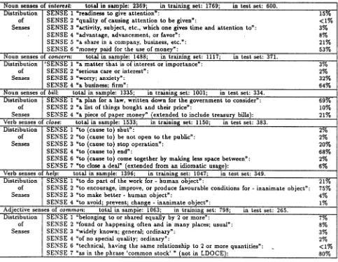
T h e training and test sets for each word selected for disambiguation were generated in the same manner. First, all instances of the word with the specified POS tag in the Penn Treebank Wall Street Journal Corpus were identified and the sentences containing them were extracted to form a d a t a sample. T h e data sample was then manually disambiguated and a test set comprising approximately one quarter of the total sample size was randomly selected. T h e size of the d a t a sample, test set, and training set for each word, along with a description of the word senses identified and their distribution in the data are presented in table 1. Table 1 also includes entries for the earlier experiments involving the noun interest

([3]).

In all of the experiments for a particular word, the estimates of the model parameters that were used were maximum likelihood estimates made from the training set for that word. In each experiment, a set of d a t a was tagged in accordance with equation (2), and the results were summarized in terms of precision and recall. (In most of the experiments, the d a t a set was the test set, as expected, b u t in the experiments de- signed to establish an upper bound for performance, it was the training set, as discussed below.) Recall is the percentage of test words that were assigned some tag; it corresponds to the portion of the test set covered by the estimate3 of the parameters made from the training set. Precision is the percentage of tagged words that were tagged correctly. A com- bined summary, the total percentage of the test set tagged correctly (the total percent correct) was also calculated.

There were three experiments run for each word. In the first, the d a t a set tagged was the test set and model M was used. In the second, the data set tagged was the test set, and the

model was the one selected using the p r o c e d u r e described in section 2 for the word being disambiguated and the contextual features used throughout the experiments. We will refer to this as the "best approximation model". In the third experiment, the data set tagged was the training set, and the model used was the one in which no assumptions are made about dependencies among variables (i.e., all variables are treated as inter-dependent). T h e purpose of experiment three was to establish upper bounds on the precision of the classifiers used in the first two experiments, as discussed in the following paragraphs.

J

If a classifier makes no assumptions regarding the dependencies among the'variables, and has available to it the actual pa- raaneter values (i.e., the true population characteristics), then the precision of that classifier would be the best that could be achieved with the specified set of features. T h e maximum likelihood estimates of the model parameters made from the training set are the population parameters for the training set; therefore, the precision of each third-experiment classifier is optimal for the training set. Because the true population will have more variation t h a n the training set, the third experiment for each word establishes an upper bound for the precision of the classifiers tested in the first two experiments for that word (and in fact, for any classifier using the same set of variables).

If we assume that the test and training sets have similar sense-tag distributions, establishing a lower bound is straight- forward. "A probabilistic classifier should perform at least as well as one that always assigns the sense that most frequently occurs in the training set. Thus, a lower bound on the precision of a probabilistic classifier is the percentage of test-word instances with the sense tag t h a t most frequently occurs.

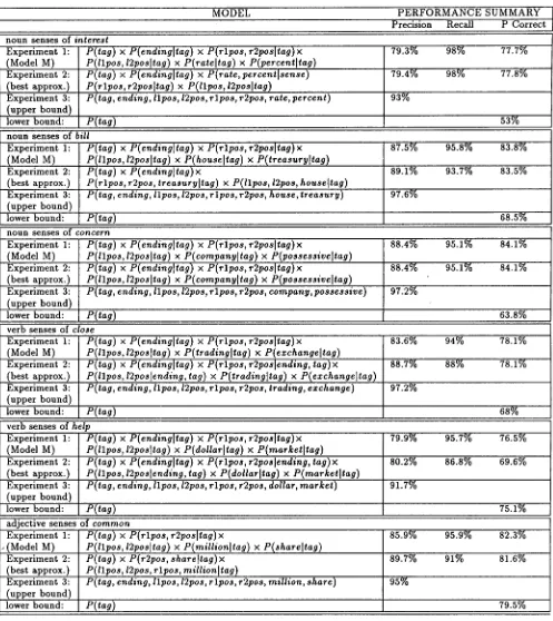
T h e results of all of the experiments, including the earlier experiments involving the noun senses of interest ([3]), are presented in table 2.

5. D I S C U S S I O N

O F R E S U L T S

In the following discussion, a classifier used in the first or second experiment for a word will be called an "experimental classifier", while a classifier used in the third experiment for a word will be referred to as the "upper-bound classifier" for that word.

Before discussing the results of the experiments, there are some comments to be made a b o u t the comparison of the performance of different classifiers. In comparing the performance of classifiers developed for the same word, it makes sense to compare the precision, recall, and total percent correct. Because the training set and the test set are the same, the differences we see are due strictly to the fact t h a t they use different models. In comparing the performance of clas- sifters developed for different words, on the other hand, only the precision measures are compared. There are two things that affect recall: the complexity of the model (i.e., the order of the highest-order marginal in the model) and the size of the training set. T h e size of the training set was not held constant for each word; therefore, comparison of the recall results for classifiers developed for different words would not be meaningful. Because total percent correct includes recall,

(4)

it should also not be used in the comparison of classifiers developed for different words.

In comparing the precision of classifiers developed for different words, what is compared is the improvement t h a t each classifier makes over the lower bound for the word for which t h a t classifier was developed.

We now turn to the specific results. Model M seems particularly well suited to the nouns (which is not surprising, given t h a t it was developed for the noun-senses of the word

interest). The precision of the noun experimental classifiers is superior to t h a t of all of the experimental classifiers developed for words in other syntactic categories. Further, for one of the nouns (concern), M was the same as the one used in experiment 2, and, for the other two nouns, M and the model used in experiment 2 are very similar.

Turning to the verbs, it is striking that, for both of the verbs, the models used in the second experiment (the best approximation models) identify an interdependency between tense markings (i.e., ending in the verb entries in table 2) and the POS tags (rlpose, r~pos, llpos, and 12pos), a dependency that is not in M. This seems to suggest t h a t a model including this dependency should be used for verbs. However, the additional complexity of such a model in comparison with M may make it less effective. For each verb we tested, a comparison of the total-percent-correct measures for experiments 1 and 2 indicates t h a t the classifier with M i s as good or b e t t e r than the classifier using the best approximation model.

The classifiers with the worst precision in comparison with the appropriate lower bound, as discussed above, are the experimental classifiers for the verb senses of help. The sense distinctions for help are based mainly on the semantic class of the syntactic object of the verb. Perhaps this approa~ch to sense disambiguation is not as effective for these kinds of sense distinctions.

Although there is a large disparity in performance between the experimental and upper-bound classifiers for a word, two things should be noted. First, the upper bounds are over- inflated due to the very small size of the training set relative to the true population (there would be much greater variation in the population). Second, such a model could never be used in practice, due to the huge number of p a r a m e t e r s to be estimated.

6 . C O N C L U S I O N S A N D F U T U R E W O R K

I n ' t h i s paper, we have presented and evaluated models created according to a schema t h a t provides a description of the joint distribution of the values of sense tags and contextual features t h a t is potentially applicable to a wide range of content words. T h e models were evaluated through a series of experiments t h a t provided the following information: 1) performance results (precision, recall, and total percent correct) for probabilistic classifiers using models created in azcordance with the schema and applied to the disambiguation of sev- eral difficult test words; 2) identification of upper and lower bounds for the performance of any probabilistic word-sense classifier using the contextual features defined in the model

schema; and 3) a comparison of the performance of classifiers using models generated per the schema to t h a t of classifiers using models selected as described in section 2. T h e results of these experiments suggest t h a t the model schema is particularly well suited to nouns b u t t h a t it is also applicable to words in other syntactic categories.

We feel t h a t the results presented in this paper are encouraging and plan to continue testing the model schema on other words. But it is unreasonable to continue generating over 1,000 manually sense-tagged examples of each word to be disambiguated, as is required if p a r a m e t e r s are estimated as we did here. In answer to this problem, other means of p a r a m - eter estimation are being investigated, including a procedure for obtaining m a x i m u m likelihood estimates from untagged data. T h e procedure is a variant of the EM algorithm ([7]) specifically applicable to models of the form described in this paper.

A C K N O W L E D G E M E N T S . T h e authors would like to gratefully acknowledge the contributions of the following people to the work presented in this paper: Rufus and Beverly Bruce for their help in sense-tagging data, Gerald Rogers for sharing his expertise in statistics, and Ted Dun- ning for advice and s u p p o r t in all m a t t e r s having to do with software development.

R e f e r e n c e s

1. Bishop, Y. M.; Fienberg, S.; and Holland, P (1975). Dis-

crete Multivariate Analysis: Theory and Practice. Cam- bridge: T h e M I T Press.

2. Brown, P.; Delia Pietra, S.; Della Pietra, V.; and Mer- cer, R. (1991). Word Sense Disambiguation Using Statis- tical Methods. Proceedings of the £9th Annual Meeting of the Association for Computational Linguistics (ACL- 91), pp. 264-304.

3. Bruce, Rebecca and Wiebe, Janyce. Word-Sense Dis- ambiguation Using Decomposable Models. Unpublished manuscript.

4. Church, K. and W. Gale (1991). A Comparison of the Enhanced Good-Turing and Deleted Estimation Meth- ods for Estimating Probabilities of English Bigrams.

Computer Speech and Language, Vol 5, pp. 19-54. 5. Church, Kenneth W and Hanks, Patrick (1990). Word

Association Norms, Mutual Information, and Lexicog- raphy, Computational Linguistics , Vol. 16, No. 1, pp. 22-29.

6. Dagan, I.; Itai, A.; and Schwall, U. (1991). Two Lan- guages Are More Informative T h a n One. Proceedings of the 29th Annual Meeting of the Association for Compu- tational Linguistics (ACL-91), pp. 130-137.

7. Dempster, A., N. Laird, and D. Rubin (1977). Maxi- mum Likelihood from Incomplete D a t a Via the EM Al- gorithm. Journal of the Royal Statistical Society B, Vol 39, pp. 1-38.

(5)

9. Havranek, T o m a s (1984). A Procedure for Model Search in Multidimensional Contingency Tables. Biometrics 40: 95-100.

10. Hearst, Mufti (1991).

Toward Noun Homonym Disambiguation--Using Local Cowtext in Large Text Corpora. Proceedings of the Sev- enth Annual Conference of the UW Centre for the New OED and Text Research Using Corpora, pp. 1-22. 11. Jelinek, F. and R. Mercer (1980). Interpolated Estima-

tion of Markov Source Parameters from Sparse Data.

Proceedings Workshop on Pattern Recognition in Prac. tice, May 21-23, Amsterdam: North-Holland.

12. Katz, S. M. (1987). Estimation of Probabilities From Sparse Data for the Language Model Component of a Speech Recognizer. IEEE Trans. Acoust., Speech, Signal Processing, Vol ASSP-35, pp. 400-401.

13. Nadas, A. (1984). Estimation of Probabilities in the Language Model of the IBM Speech Recognition Sys- tem. IEEE Trans. Acoust., Speech, Signal Processing,

Vol ASSP-32, pp. 859-861.

14. Yarowsky, David (1992). Word-Sense.Disambiguating Using Statistical Models of Roget's Categories Trained on Large Corpora. Proceedings of the 15th International Conference on Computational Linguistics (COLING- 9e).

15. Yarowsky, David (1993). One Sense Per Collocation.

Proceedings of the Speech and Natural Language ARPA Workshop, March 1993, Princeton, NJ.

16. Zernik, Uri (1990). Tagging Word Senses In Corpus: The Needle in the Haystack Revisited. Technical Report 90CRDI98, GE Research and Development Center.

Distribution of Senses

S E N S E 1 "readiness to give attention": 1 5 % S E N S E 2 "quality of causing attention to be given": < 1 % SENSE 3 %ctivity, subject, etc., wh{ch one gives time and attention t o ' : 3%

SENSE 4 "advantage, advancement, or favor": 8%

SENSE 5 "a share in a company, business, etc.": 21%

SENSE 6 "money paid for the use of money": 53%

N o u n senses of concern: total in sample: 1488; in training set: 1117; in test set: 371.

Distribution ~ S E N S E 1 "a matter that is of interest or importance': 3 %

of S E N S E 2 "serious caxe or interest": 2 %

Senses SENSE 3 ~worry; anxiety": 32%

SENSE 4 "a business; firm": 64%

Noun senses of bill: total in sample: 1335; in training set: 1001; in test set: 334.

Distribution S E N S E 1 "a plan for a law, written d o w n for the government to consider": 69%" of S E N S E 2 "a list of things bought and their price": 1 0 % Senses SENSE 4 "a piece of paper money" !extended to include treasury bills~: 21% Verb senses of

S E N S E 1 "to (cause to) shut": 2~0

S E N S E 2 "to (cause to) be not open to the public": 2 % S E N S E 3 "to (cause to) stop operation": 2 0 %

S E N S E 4 "to (cause to) end": 6 8 %

SENSE 6 "to (cause to) come together by making less space between": 2% SENSE 7 "to close a deal" (extended from an idiomatic usage): 6% Verb senses of help: total in sample: 1396; in training set: 1047; in test set: 349.

Distribution S E N S E i "to do part of the work for - h u m a n object": 2 1 % of S E N S E 2 "to encourage, improve, or produce favourable conditions for - inanimate object": 7 5 % Senses S E N S E 3 "to m a k e better - h u m a n object": 4 %

S E N S E 4 ~to avoid; prevent; change - inanimate object": 1 % Adjective senses of c o m m o n : total in sample: 1063; in training set: 798; in test set: 265.

S E N S E 1 "belonging to or shared equally by 2 or more":

S E N S E 2 ~found or happening often and in m a n y places; usual": S E N S E 3 "widely known; general; ordinary":

S E N S E 4 "of no special quality; ordinary~:

S E N S E 6 ~technical, having the s a m e relationship to 2 or more quantities': S E N S E 7 "as in the phrase ' c o m m o n stock' " (not in L D O C E ) :

7% 8% 3% 2% <1% 80%

Table 1: Data summary.

[image:5.612.72.555.289.663.2]

(6)

MODEL PERFORMANCE SUMMARY Precision Recall P Correct noun senses of

Experiment 1: (Model M) Experiment 2: (best approx.) Experiment 3: (upper bound) lower bound:

interest

P(tag) x P(endingltag ) x P(rlpos, r2posltag)x

P(llpos, 12posltag) x P(rateltag) x P(percentttag)

P(tag) x P(ending]tag) x P(rate,percentlsense )

P(rlpos, r2posltag ) x P(llpos, 12posltag )

! P(tag, ending, llpos, 12pos, rlpos, r2pos, rate, percent)

P(tag)

79.3% 98% 77.7%

79.4% 98% 77.8%

93%

53%

n o u n s e n s e s o f Experiment 1: (Model M) Experiment 2: (best approx.) Experiment 3: (upper bound) lower bound:

bill

P(llpos, 12posltag) x P(houseltag) x P(treasuryltag )

P(tag) x P(endingltag)x

P(rlpos, r2pos, treasuryltag ) x P(llpos, 12pos, house]tag)

P( tag, ending, ll pos, 12pos, r l pos, r2pos, house, treasury)

P(tag)

87.5% 95.8% 83.8%

89.1%

97.6%

93.7% 83.5%

68.5% noun senses of

concern

P(llpos, 12posltag) x P(companyltag ) x P(possessiveltag )

P(llpos, 12posltag) x P(companyltag ) x P(possessiveltag)

P( tag, ending, ll pos, 12pos, r l pos, r2pos, company, possessive)

P(tag)

88.4%

97.2%

95.1% 84.1%

63.8% verb senses of

close

P(tag) x P(ending]tag) x P(rlpos, r2pos[tag) x

P(llpos, 12pos[tag) x P(tradingltag) x P(ezchangeltag)

P(tag) x P(cnding]tag) x P(rlpos, r2pos[ending, tag)x

P(llpos, 12poslending, tag) x P(tradingltag) x P(ezchangeltag )

P( tag, ending, llpos, 12pos, rlpos, r2pos, trading, exchange)

P(tag)

83.6% 94% 78.1%

88.7% 88% 78.1%

97.2%

68% verb senses of

help

P(tag) x P(endingltag) x P(rlpos, r2posltag)x

P(llpos, 12posltag) x P(dollarltag)

x

P(marketltag )

P( tag) x P(ending]tag) x P(r lpos, r2poslending , tag) x

P(llpos, t2poslending, tag) × P(dollarltag) x P(marketltag)

P( tag, ending, llpos, 12pos, r lpos, r2pos, dollar, market)

P(tag)

79.9% 95.7% 76.5%

80.2%

91.7%

86.8% 69.6%

75.1% adjective senses of

common

Experiment 1: .(Model M)

Experiment 2: (best approx.) Experiment 3: (upper bound) lower bound:

P(tag) x P(rlpos, r2posltag) x

P(llpos, 12posltag ) x P(millionltag ) x P(shareltag )

P(tag) x P(r2pos, shareltag) x

P( llpos, 12pos, r lpos, millionltag )

P( tag, ending, llpos, 12pos, r lpos, r2pos, million, share)

P(tag)

85.9% 95.9% 82.3%

89.7%

95%

91% 81.6%

79.5%

Table 2: Results of experiments.

[image:6.612.64.561.42.600.2]