A context-based model for Sentiment Analysis in Twitter
Andrea Vanzo and Danilo Croce and Roberto Basili Department of Enterprise Engineering
University of Roma Tor Vergata Via del Politecnico 1, 00133 Roma Italy
{vanzo,croce,basili}@info.uniroma2.it
Abstract
Most of the recent literature on Sentiment Analysis over Twitter is tied to the idea that the senti-ment is a function of an incoming tweet. However, tweets are filtered through streams of posts, so that a wider context, e.g. a topic, is always available. In this work, the contribution of this contextual information is investigated. We modeled the polarity detection problem as a sequen-tial classification task over streams of tweets. A Markovian formulation of the Support Vector Machine discriminative model as embodied by theSVMhmmalgorithm has been here employed to assign the sentiment polarity to entire sequences. The experimental evaluation proves that se-quential tagging effectively embodies evidence about the contexts and is able to reach a relative increment in detection accuracy of around 20% in F1 measure. These results are particularly interesting as the approach is flexible and does not require manually coded resources.
1 Introduction
Since in the Web 2.0 users can write about their life, personal experiences, share contents about facts and ideas, Social Networks became valuable sources of opinions and sentiments. This huge amount of data is crucial in the study of the interactions and dynamics of subjectivity on the Web, largely relevant for marketing tasks. Twitter is one among these microblogging services that counts about a billion of active users and 500 million of daily messages1. However, the analysis of this huge amount of information is
still challenging, as language is very informal, affected by misspelling and characterized by slang and
#hashtags, i.e. special user-generated tags used to contextualize different tweets around a specific topic. Researches focused on the computational study and automatic recognition of opinions and sentiments as they are expressed in free texts. It gave rise to what is currently known as Sentiment Analysis, a set of tasks aiming to detect the subjective attitude of a writer with respect to some topic. Many Sentiment Analysis studies map sentiment detection in a Machine Learning(ML) setting (Pang and Lee, 2008), where labeled data, i.e. known examples, allow to induce the detection function from real world exam-ples. In general, sentiment detection in tweets has been generally treated as any other text classification task, as proved by most papers participating to theSentiment Analysis in Twittertask in SemEval-2013 challenge (Nakov et al., 2013): a computational representation for an incoming instance is generated by just considering one tweet at a time. The short length of the message and the resulting semantic ambi-guity are critical limitations and make the task very complex. Let us consider the following example, in which a tweet fromColMustardcitesSergGray:
ColMustard : @SergGray Yes, I totally agree with you about the substitutions! #Bayern #Freiburg
The tweet sounds like to be a reply to the previous one. Notice how no lexical nor syntactic property allows to determine the sentiment polarity. However, if we look at the entire conversation that follows:
ColMustard: Amazing match yesterday!!#Bayern vs. #Freiburg 4-0 #easyvictory
SergGray: @ColMustard Surely, but #Freiburg wasted lot of chances to score.. wrong substitutions by #Guardiola during the 2nd half!!
ColMustard: @SergGray Yes, I totally agree with you about the substitutions! #Bayern #Freiburg
This work is licenced under a Creative Commons Attribution 4.0 International License. Page numbers and proceedings footer are added by the organizers. License details:http://creativecommons.org/licenses/by/4.0/
1http://expandedramblings.com/
it is easy to establish that a first positive tweet has been produced, followed by a second negative one so that the third tweet is negative as well. It is the conversation that allows us here to disambiguate even a very short message and properly characterize it according to its author and posting time.
We want here to capitalize such a richer set of observations (i.e. entire conversations) and to define a context-sensitive SA model along two lines: first, by enriching a tweet representation to include the conversation information, and then introducing a more complex classification model that works over an entire tweet sequence and not on one tweet (i.e. the target) at a time. Accordingly, in the paper we will first focus on different representations of tweets that can be made available to the sentiment detection process. They will also account for contexts, that areconversations, as chains of tweets that are reply to the previous ones, andtopics, built around hashtags. These are in fact topics made explicit by users, such as events (#easyvictory) or people (#Guardiola). It represents a wider notion of conversation that enforces the sense of belonging to a community. From a computational perspective, the polarity detection of a tweet in a context is here modeled as a sequential classification task. In fact, both conversation and topic-based context are arbitrarily long sequences of messages, ordered according totimewith the target tweet being the last. The SVMhmm learning algorithm (Altun et al., 2003) has been employed, as it allows to classify an instance (here, a tweet) within an entire sequence. While SVM based classifiers allow to recognize the sentiments from one specific tweet at a time, the SVMhmm learning algorithm collectively labels all tweets in a sequence. It is thus expected to capture patterns within a conversation and apply them in novel sequences, through a standard decoding task.
While all the above contexts extend a tweet representation, they are still local to a specific notion of conversation. In this work, we also explore the somehow more abstract notion of contexts given by the emotional attitude shown by each user in his overall usage of Twitter. In the above example, ColMustardshows a specific attitude while discussing about the Bayern Munchen. We can imagine that this feature characterizes most of its future messages at least about football. We suggest to enrich the tweet representation with features thatsynthesize a user’s profile, in order to catch possible biases towards a particular sentiment polarity. This is quite interesting as it has been shown that communities behave in a coherent way and users tend to take stable standing points. Experimental evaluation (Chapter 4) proves the effectiveness of this proposed sequential tagging approach combined with the adopted contextual information, improving the percentage of correctly recognized tweets up to 12%.
A survey of the existing approaches is presented into Section 2. Then, Section 3 provides an account of the context-based models: conversation, topic-based and user sentiment profiling. The experimental evaluation into Section 4 prove the positive impact of social dynamics on the SA task.
2 Related Work
Sentiment Analysis has been described as aNatural Language Processingtask at many levels of gran-ularity. Starting from being mapped into adocument level classification task (Turney, 2002; Pang and Lee, 2004), it has been also applied atsentence level(Hu and Liu, 2004; Kim and Hovy, 2004) and more recently at thephrase level(Wilson et al., 2005; Agarwal et al., 2009).
2010; Agarwal et al., 2011; Castellucci et al., 2013), are mostly employed. An interesting perspective, where a kind of contextual information is studied, is presented in (Mukherjee and Bhattacharyya, 2012): the sentiment detection of tweets is here modeled according to lexical features as well as discourse relations like the presence of connectives, conditionals and semantic operators likemodalsandnegations. Nevertheless, in all the above approaches, features are derived only from lexical resources or from the tweet itself and no contextual information is exploited. However, given one tweet targeted for sentiment detection, more awareness about its content is available to writers and readers by the entire stream of related posts immediately preceding it. In order to exploit this wider information, a Markovian extension of a Kernel-based categorization approach is proposed in the next section.
3 A context based model for Sentiment Analysis in Twitter
As discussed in the introduction, contextual information about one tweet stems from various aspects: an explicit conversation, the user attitude or the overall set of recent tweets about a topic (for example an hastag like#Bayern). As individual perspectives on the context are independent (a conversation may or may not depend on user preference or cheer) and they also obey to different notion of analogies or similarity, we should avoid a unified feature vector, but employ independent representations. A structured view on a tweet can thus be provided by considering it as multifaceted entity where a set of vectors, each one contributing to one aspect of the overall representation, exhibits a specific similarity metrics. Notice how this is exactly what Kernel-based learning supports, whereas the combination of the different Kernel functions can be easily made a Kernel function itself (Shawe-Taylor and Cristianini, 2004). Kernel functions are used to capture specific aspects of the semantic relatedness between two tweets and are easily integrated in various Machine Learning algorithms, such as SVM.
3.1 Representing tweets through different Kernel functions
Many Machine Learning approaches for Sentiment Analysis in Twitter benefited by complex ways of modeling of individual tweets, as discussed in many works (Nakov et al., 2013). The representation we propose makes use of individual Kernels as models of different aspects usable within a SVM paradigm.
Bag of Word Kernel (BoWK). The simplest Kernel function describes the lexical overlap between tweets, thus represented as vectors, whose dimensions correspond to the different words. Components denote the presence or not of the corresponding word in the text and Kernel function corresponds to the cosine similarity between vector pairs. Even if very simple, the BoW model is one of the most informative representation in Sentiment Analysis, as emphasized since (Pang et al., 2002).
Lexical Semantic Kernel (LSK). Lexical information in tweets can be very sparse, as we will also show in the next Section 4. In order to extend the BoW model, we provide a further vector representation aiming to generalize the lexical information. It can be obtained for every term of a dictionary by a co-occurrence Word Space built according to the Distributional Analysis described in (Sahlgren, 2006). A word-by-context matrix, M, is built through large scale corpus analysis and then processed through
Latent Semantic Analysis(Landauer and Dumais, 1997). The dimensionality of the space represented by
Mcan be reduced through Singular Value Decomposition (SVD) (Golub and Kahan, 1965). The original statistical information aboutM is captured by the newk-dimensional space, which preserves the global structure while removing low-variance dimensions, i.e. distribution noise. The result is that every word is projected in the reduced Word Space and a vector for each tweet is represented through the linear combination of the co-occurring word vectors (also calledadditive linear combinationin (Mitchell and Lapata, 2010)). The resulting Kernel function is thecosine similaritybetween tweet vector pairs, in line with (Cristianini et al., 2002). Notice that the adoption of a distributional approach does not limit the overall application, as it can be automatically applied without relying on any manually coded resource.
User Sentiment Profile Context(USPK). A source of evidence about a tweet is its author, with his attitude towards some polarities. Specific features based on the users’ previous tweets can be derived as follows. Letti∈ T be a tweet andi∈N+its identifier. TheUser Profile Context(Ui) can be defined as the set of the lastHtweets posted by the author ofti, hereafter denoted byui. This information is a body of evidence about the opinion holder’s profile on which a further tweet representation can be defined. A tweettiis here mapped into a three dimensional vector~µi = µ1i, µ2i, µ3i
the indicator of polarity inclination, i.e.positive,negativeandneutral, expressed through the conditional probabilityP(j | ui)for the polarity labels j ∈ Y given the user ui. We can suppose that, for each
tk∈Ui, its corresponding labelykis available either as a gold standard annotation or predicted in a semi-supervised fashion by trained classifiers. The estimation ofµji ≈P(j|ui), is aσ-parameterizedLaplace
smoothed versionof the observations inUi:µji =Pk|U=1i|(1{yk=j}(tk) +σ)/(|Ui|+σ|Y|)whereσ ∈R is the smoothing parameter, j ∈ Y, i.e. the set of polarity labels. The Kernel function, called User Sentiment Profile Kernel (USPK), is thecosine similaritybetween two vectors(~µi, ~µm).
The multiple Kernel approach. Whenever the different Kernels are available, we can apply a lin-ear combinationαBoWK+βLSK orαBoWK+βLSK+γUSPK in order to exploit lexical and semantic properties captured by BoWK and LSK, or user properties as captured by USPK.
3.2 Modeling tweet conversation as a sequential tagging problem
The User Sentiment Profile Kernel (UPSK) can be seen as an implicit representation of a context de-scribing the writer. However, contextual information is usually embodied by the stream of tweets in which the target onetiis immersed. Usually, the stream is something available to a reader and includes an entireconversation(where links to the previous tweets are made explicit and are supposed to be all available) or atopic, i.e. a hashtag, the reader has searched for. In all cases, the stream give rise to an entire sequence on which sequence labeling can be applied: the target tweet is here always labeled within the entire sequence, where contextual constraints are provided by the preceding tweets. More formally, two types of context are defined:
Conversational context. For every tweetti ∈ T, letr(ti) :T → T be a function that returns either the tweet to whichti is a reply to, ornullifti is not a reply. Then, theconversation-based contextΛC,li of tweetti(i.e., thetarget tweet) is the sequence of tweet iteratively built by applyingr(·), untilltweets have been selected orr(·) = null. In other words, lallows to limit the size of the input context. An example of conversation-based context is given in Section 1.
Topical context.Hashtags allow to aggregate different tweets around a specific topic. An entire tweet sequence can be derived including thentweets preceding the targettithat contain the same hashtag set. This is usually the output of a search in Twitter and it is likely the source information that influenced the writer’s opinion. Letti ∈ T be a tweet andh(i) : T → P(H) be a function that returns the entire hashtag setHi ⊆ Hobserved into ti. Then, thehashtag-based context ΛH,li for a tweetti (i.e.,target
tweet) is a sequence of the most recentltweetstjsuch thatHj∩Hi 6=∅, i.e.tj andtishare at least one hashtag, andtj has been posted beforeti. As an example, the following hashtag-based context of size 4 has been obtained about#Bayern:
MrGreen: Fun fact: #Freiburg is the only #Bundesliga team #Pep has never beaten in his coaching career. #Bayern MrsPeacock: Young starlet Xherdan #Shaqiri fires #Bayern into a 2-0 lead. Is there any hope for #Freiburg?
pic.twitter.com/krzbFJFJyN
ProfPlum: It is clear that #Bayern is on a rampage leading by 4-0, the latest by Mandzukic... hoping for another 2 goals from #bayernmunich
MissScarlet: Noooo! I cant believe what #Bayern did!
It is clear thatMissScarletexpressed an opinion, but the corresponding polarity is easily evident when the entire stream is available about the#Bayernhashtag. As well as in a conversational context, a specific context sizencan be imposed by focusing only on the lastntweets of the sequence. Once different representations and contexts are available a structured learning-based approach can be applied to Sentiment Analysis. Firstly, we will discuss a discriminative learning approach that follows the multi-classification schema proposed in (Joachims et al., 2009), namely SVMmulticlass . Then a sequence labeling approach, based on theSVMhmmlearning algorithm (Altun et al., 2003), will be introduced, as an explicit account of bothconversationalandtopicalcontexts.
The multi-class approach.TheSVMmulticlassschema described in (Joachims et al., 2009) is applied2
to implicitly compare all polarity labels and select the most likely one, using the multi-class formulation described in (Crammer and Singer, 2001). The algorithm thus acquires a specific function fy(x) for
each sentiment polarity labely∈ Y, whereY ={positive, negative, neutral}. Given a feature vector
x∈ X representing a tweetti,SVMmulticlassallows to predict a specific polarityy∗ ∈ Yby applying the discriminant functiony∗ = arg max
y∈Yfy(xi), wherefy(x) =wy·xis a linear classifier associated to each labely. Given a training set(x1, y1). . .(xn, yn), the learning algorithm determines each classifier parameterswyby solving the following optimization problem:
min12 X
i=1...k
kwik2+C
n X
i=1...n
ξi s.t.∀i,∀y∈ Y:xi·wyi≥xi·wy+ 100∆(yi, y)−ξi
whereCis a regularization parameter that trades off margin size and training error, while∆(yi, y)is the loss function that returns0ifyiequalsy, and1otherwise.
The markovian approach. The sentiment prediction of a target tweet can be seen as a sequential classification task over a context, and the SVMhmm algorithm can be thus applied. Given an input sequencex= (x1. . . xl)⊆ X, wherexis a tweet context, e.g. theconversationaland thehashtag-based one (i.e. ΛC,li andΛH,li , respectively) andxiis a feature vector representing a tweet, the model predicts a tag sequencey= (y1. . . yl)∈ Y+after learning a linear discriminant functionF :P(X)× Y+→R over input/output pairs. The labelingf(x) is thus defined as: f(x) = arg maxy∈Y+F(x,y;w). It is obtained by maximizingF over the response variable,y, for a specific given input,x. In these models,
F is linear in some combined feature representation of inputs and outputsΦ(x,y), i.e. F(x,y;w) =
hw,Φ(x,y)i. AsΦextracts meaningful properties from an observation/label sequence pair (x,y), in
SVMhmmit is modeled through two types of features: interactions between attributes of the observation vectorsxiand a specific labelyi(i.e. emissionsofxibyyi) as well as interactions between neighboring labelsyi along the chain (transitions). In other words,Φis defined so that the complete labelingy =
f(x)can be computed efficiently fromF, using aViterbi-like decoding algorithm, according to the linear discriminant function
y∗ = arg max
y∈Y+ {
X
i=1...l
[ X
j=1...k
(xi·wyi−j... yi) + Φtr(yi−j, . . . , yi)·wtr]}
In the training phase, SVMhmm solves the following optimization problem given training examples (x1,y1). . .(xn,yn)of sequences of feature vectorsxj with their correct tag sequencesyj
min 12kwk2+C
n X
i=1...n
ξi
s.t. ∀y, n: { X
i=1...l (xn
i ·wyn
i) + Φtr(y
n
i−1, yni)·wtr} ≥ { X i=1...l
(xn
i ·wyi) + Φtr(yi−1, yi)·wtr}+ ∆(yn, y)
where ∆(yn, y) is the loss function, computed as the number of misclassified tags in the sequence, (xi·wyi)represents the emissions andΦtr(yi−1, yi)the transitions. Indeed, throughSVMhmmlearning the label for the target tweet is made dependent on its context history. The markovian setting thus acquires patterns across tweet sequences to recognize sentiment even for truly ambiguous tweets. 4 Experimental Evaluation
The aim of the experiments is to estimate the contribution of the proposed contextual models to the accuracy reachable in different scenarios, whereas rich contexts (e.g. popular hashtags) are possibly made available or just singleton tweets, with no context, are targeted.
We adopted the “Sentiment Analysis in Twitter” dataset3 as it has been made available in the ACL SemEval-2013 (Nakov et al., 2013). However, in order to rely on tweet identifiers (needed to retrieve contexts from Twitter servers), only the Training and Development portions of the data (11,338 exam-ples), for which id’s were made available, have been employed. As about 10,045 tweets were available from the servers,4a static split 80/10/10 inTraining/Held-out/Testrespectively, has been carried out as
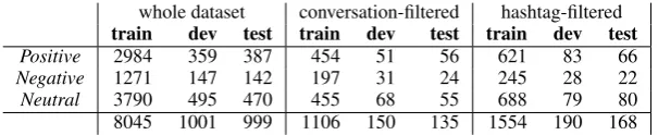
reported in Table 1. As the performance evaluation is always carried out against one target tweet (in analogy with the benchmark of SemEval-2013), the multi-classification may happen when no context is available (i.e. there is no conversation nor hashtag to built the context from) or when a rich conversa-tional or topical context is available. In Table 1 different datasets are shown in columns 2-4, 5-7 and 8-10
3http://www.cs.york.ac.uk/semeval-2013/task2/index.php?id=data
respectively: the entire corpus of 10,045 is represented in columns 2-4, while 5-7 and 8-10 represents the subsets of target tweets for which a conversational or topical context, respectively, was available. Conversational contexts are available only for 1,391 tweets (columns 5-7), while hashtag-based contexts include 1,912 instances (columns 8-10).
whole dataset conversation-filtered hashtag-filtered
train dev test train dev test train dev test
Positive 2984 359 387 454 51 56 621 83 66
Negative 1271 147 142 197 31 24 245 28 22
Neutral 3790 495 470 455 68 55 688 79 80
[image:6.595.147.450.123.185.2]8045 1001 999 1106 150 135 1554 190 168
Table 1: Whole dataset composition
As tweets are noisy texts, a pre-processing phase has been applied to improve the quality of linguistic features observable and reduce data sparseness. In particular, a normalization step is applied to each post: fully capitalized words are converted in lowercase; reply marks are replaced with the pseudo-token USER, hyperlinks byLINK,hashtagsby HASHTAGand emoticons by special tokens5. Afterwards, an
almost standard NLP chain is applied through theChaosparser (Basili et al., 1998; Basili and Zanzotto, 2002). In particular, each tweet, with its pseudo-tokens produced by the normalization step, is mapped into a sequence of POS tagged lemmas. Emoticons are treated as nouns. In order to feed the LSK, lexical vectors correspond to a Word Space derived from a corpus of about 1.5 million tweets, downloaded during the experimental period and using the topic names from the trial material as query terms. Every wordwin such corpus is represented as one co-occurrence vector as in (Sahlgren, 2006) with the setting discussed in (Croce and Previtali, 2010): left and right co-occurrence scores are obtained in a window of sizen=±5around eachw. Vector componentswf correspond to Pointwise Mutual Information values
pmi(w, f)between the wordw(the row) and the featuref. Dimensionality reduction is applied to the co-occurrence matrix, through SVD, with a dimensionality cut ofk= 250.
Existing state-of-the-art approaches neglect the tweet context, so that datasets with labeled contexts are not available: USPK or the markovian approach would not be applicable. The solution consisted in creating a semi-supervised Gold-Standardby training the multi-class classifier (not employing any context) fed through a combination of BoWK and LSK Kernel functions and get the classification of all tweets within the context of at least one target tweet. Unfortunately, this can introduce noise, but it is a realistic solution to a cold-start approach, easily portable to other datasets.
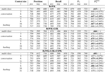
Performance scores report the classification accuracy in terms of Precision, Recall and standard F-measure. However, in line with SemEval-2013, we also report theF1pnnscore as the arithmetic mean between theF1s ofpositive,negativeandneutralclasses.
4.1 Experiment 1: Using contexts in a general tweet classification setting
A first experiment has been run to validate the impact of contextual information over generic tweets, independently from the availability of the context. In this case, the entire data set is used. The different settings adopted are reported in independent rows, corresponding to different classification approaches:
• multi-classrefers to the application of the multi-classification ofSVMmulticlass, that does not require any context and can be considered as a baseline for the employed Kernel combinations;
• conversationrefers to theSVMhmmclassifier observing the conversation-based contexts. The train-ing and testtrain-ing of the classifier is here run with differentcontext sizes, by parameterizinglinΛC,li ;
• likewise,hashtagrefers to theSVMhmmclassifier observing the topic-based contexts, when hash-tags are considered. Differentcontext sizes have been considered, by parameterizinglinΛH,li . In bothconversationandhashtagmodels, when no context is available, theSVMhmmclassifier acts on a sequence of length one, and no transition is used. Table 2 shows the empirical results over the whole test dataset. The first general outcome is that algorithmic baselines, i.e. context-free models that use no contextual information, in the multi-class rows are better performing whenever richer representations are provided. The LSA information (+8.29%) as well as the user profiling (+10.73%) seem beneficial in
Context size Precision Recall F1 Fpnn1
l pos neg neu pos neg neu pos neg neu
BoWK
multi-class - .713 .496 .680 .649 .401 .770 .679 .444 .723 .615( - ) conversation 36 .761.728 .493.500 .695.718 .651.677 .465.479 .768.789 .701.702 .489.478 .742.739 .644 (.640 (+4.72%+4.07%))
∞ .723 .511 .722 .695 .472 .762 .709 .491 .741 .647 (+5.20%)
hashtag
3 .766 .533 .675 .633 .401 .821 .693 .458 .741 .631 (+2.60%) 6 .727 .575 .711 .682 .514 .770 .704 .543 .740 .662 (+7.64%) 16 .717 .561 .730 .693 .549 .755 .704 .555 .743 .667 (+8.46%)
31 .717 .533 .738 .705 .570 .732 .711 .551 .735 .666 (+8.29%)
BoWK+LSK
multi-class - .754 .595 .704 .674 .486 .804 .712 .535 .751 .666( - ) conversation 36 .759.760 .595.536 .712.737 .682.713 .486.521 .781.811 .736.718 .529.535 .758.758 .674 (.670 (+1.20%+0.60%))
∞ .774 .554 .717 .682 .542 .791 .725 .548 .752 .675 (+1.35%)
hashtag
3 .731 .541 .737 .729 .556 .732 .730 .549 .734 .671 (+0.75%) 6 .770 .580 .736 .700 .585 .789 .733 .582 .762 .693 (+4.05%)
16 .742 .519 .732 .693 .570 .751 .717 .544 .742 .667 (+0.15%) 31 .751 .537 .729 .685 .556 .774 .716 .547 .751 .671 (+0.75%)
BoWK+LSK+USPK
multi-class - .778 .612 .716 .680 .500 .830 .726 .550 .768 .681( - ) conversation 63 .771.753 .563.654 .689.707 .625.693 .507.493 .806.817 .721.690 .562.533 .753.748 .679 (-0.29%).657 (-3.67%)
∞ .767 .566 .713 .690 .514 .791 .727 .539 .750 .672 (-1.32%)
hashtag
3 .753 .556 .735 .693 .599 .766 .721 .576 .750 .683 (+0.29%) 6 .747 .594 .735 .711 .556 .779 .728 .575 .756 .686 (+0.73%)
[image:7.595.84.514.61.356.2]16 .742 .519 .742 .700 .592 .745 .721 .553 .743 .672 (-1.32%) 31 .738 .530 .739 .693 .556 .766 .715 .543 .752 .670 (-1.62%)
Table 2: Evaluation results on whole dataset.
their relative improvements with respect to the simple BoW Kernel accuracy. Second, almost all context-driven models (i.e.SVMhmmoperating on different context sizes) improvewrttheirSVMmulticlass coun-terpart. Every polarity category benefits from the introduction of contexts, although this is particularly true for the negative (neg) case, where a 15.5% of the entire dataset examples are available: it seems clear that contexts allow to compensate against poor training conditions.
4.2 Experiment 2: Measuring the full impact of context-based models over rich contexts
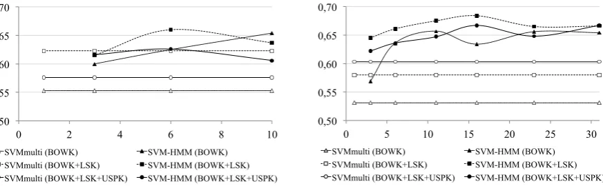
Given the above outcomes, a second set of experiments has been run against the subset of the test data restricted to tweets for which rich contexts are available, as introduced in Table 1. In Figure 1, the per-formances of different learning paradigms and Kernels trained and tested over these corpora are shown. On the Left of the figure, the performance over the conversation-filtered corpus (Table 1) are reported: these tweets are characterized by rich conversational contexts of different increasing sizes on the X-axis. On the Right of Figure 1, the corresponding performances obtained over the hashtag-filtered corpus are reported. As the number of available examples in both test corpora is much smaller, the baselines corresponding to theSVMmulticlassapproach are lower.
On the contrary, such poorer training evidence does not seem to afflict the contextual models in both corpora, as the markovian modeling seems to bring a straight benefit. In particular, increasing amount of contextual information is usually beneficial to accuracy scores. In general, theSVMhmmaccuracy plots seem to increase up to a given context size, that is around 6 for conversational contexts vs. 16 previous tweets for topical contexts. It seems that a wider context (i.e. a window of 8 or 10 tweets) is not so beneficial, as the generalization emphasized by LSK and USPK tends to diverge. Different genres of discussions seem to provide different useful contexts for sentiment detection. The overall benefit reach-able bySVMhmm relatively to theSVMmulticlass baseline is striking as only rich contexts are used for training and testing. The BoW Kernel over the conversation corpus has an overall relative improvement of 18.26% inF1pnn, where the richer BoWK+LSK Kernel improves of about 5.94%. Boosts inF1pnn
0,50 0,55 0,60 0,65 0,70
0 2 4 6 8 10
SVMmulti (BOWK) SVM-HMM (BOWK) SVMmulti (BOWK+LSK) SVM-HMM (BOWK+LSK) SVMmulti (BOWK+LSK+USPK) SVM-HMM (BOWK+LSK+USPK)
0,50 0,55 0,60 0,65 0,70
0 5 10 15 20 25 30
[image:8.595.80.517.77.212.2]SVMmulti (BOWK) SVM-HMM (BOWK) SVMmulti (BOWK+LSK) SVM-HMM (BOWK+LSK) SVMmulti (BOWK+LSK+USPK) SVM-HMM (BOWK+LSK+USPK)
Figure 1: TheF1pnnmeasure of the different classifiers vs. different context sizes. On the Left: perfor-mances when conversational contexts are employed. On the Right: topical contexts are adopted.
BOWK+LSK into the markovian approach, seems to not provide any useful contribution. A clash be-tween the global information (as modeled by the USPK) and the local information (embedded in the recent tweets about a topic) is here observed: when these enter in an opposition, the contrast penalizes the accuracy of the linear combination of Kernels. In general, the improvements implied by contextual information are related to the treatment of particularly ambiguous tweets. In a conversation, such as
MrGreen: Cannot wait to meet @therealjuicyj and @RealWizKhalifa with @Hill Gonzz
November 29th #trippyniqqas (positive)
ColMustard: @MrGreen where they gone be?? (neutral)
MrGreen: @ColMustard New Orleans!!! (positive)
ColMustard: @MrGreen house of blues? (neutral)
MrGreen: @ColMustard no it’s at the UNO lakefront arena (neutral)
ColMustard: @MrGreen I’m going Tuesday to the house of blues to see ASAP Rocky (neutral) the switch to aneutralmode characterizing the target tweet is a consequence of the entire sequence and captured as a pattern. The contribution of the topical contexts is finally evident in the following example:
... ... ... ... ... ...
ProfPlum: Can’t wait to get out there with my boys Go Team! #goeagles (positive)
MrsPeacock: GO my awesome team @WestCoastEagles!!!!! #goeagles #weflyhigh :D (positive)
MissScarlet: Let’s go eagles :) #goeagles (positive)
SergGray: keen for the eagles game today. #goeagles (positive) 5 Conclusions
References
Apoorv Agarwal, Fadi Biadsy, and Kathleen R. Mckeown. 2009. Contextual phrase-level polarity analysis using lexical affect scoring and syntactic n-grams. InProceedings of the 12th Conference of the European Chapter of the Association for Computational Linguistics, EACL ’09, pages 24–32, Stroudsburg, PA, USA. Association for Computational Linguistics.
Apoorv Agarwal, Boyi Xie, Ilia Vovsha, Owen Rambow, and Rebecca Passonneau. 2011. Sentiment analysis of twitter data. InProceedings of the Workshop on Languages in Social Media, LSM ’11, pages 30–38, Strouds-burg, PA, USA. Association for Computational Linguistics.
Y. Altun, I. Tsochantaridis, and T. Hofmann. 2003. Hidden Markov support vector machines. InProceedings of the International Conference on Machine Learning.
Luciano Barbosa and Junlan Feng. 2010. Robust sentiment detection on twitter from biased and noisy data. In Chu-Ren Huang and Dan Jurafsky, editors,COLING (Posters), pages 36–44. Chinese Information Processing Society of China.
Roberto Basili and Fabio Massimo Zanzotto. 2002. Parsing engineering and empirical robustness. Nat. Lang. Eng., 8(3):97–120, June.
Roberto Basili, Maria Teresa Pazienza, and Fabio Massimo Zanzotto. 1998. Efficient parsing for information extraction. InProc. of the European Conference on Artificial Intelligence, pages 135–139.
Albert Bifet and Eibe Frank. 2010. Sentiment knowledge discovery in twitter streaming data. InProceedings of the 13th International Conference on Discovery Science, DS’10, pages 1–15, Berlin, Heidelberg. Springer-Verlag.
Giuseppe Castellucci, Simone Filice, Danilo Croce, and Roberto Basili. 2013. Unitor: Combining syntactic and semantic kernels for twitter sentiment analysis. In Second Joint Conference on Lexical and Computational Semantics (*SEM), Volume 2: Proceedings of the Seventh International Workshop on Semantic Evaluation (SemEval 2013), pages 369–374, Atlanta, Georgia, USA, June. Association for Computational Linguistics. K. Crammer and Y. Singer. 2001. On the algorithmic implementation of multi-class svms. Journal of Machine
Learning Research, 2:265–292.
Nello Cristianini, John Shawe-Taylor, and Huma Lodhi. 2002. Latent semantic kernels. J. Intell. Inf. Syst., 18(2-3):127–152, March.
Danilo Croce and Roberto Basili. 2012. Grammatical feature engineering for fine-grained ir tasks. In Giambattista Amati, Claudio Carpineto, and Giovanni Semeraro, editors,IIR, volume 835 ofCEUR Workshop Proceedings, pages 133–143. CEUR-WS.org.
Danilo Croce and Daniele Previtali. 2010. Manifold learning for the semi-supervised induction of framenet pred-icates: An empirical investigation. InProceedings of the 2010 Workshop on GEometrical Models of Natural Language Semantics, GEMS ’10, pages 7–16, Stroudsburg, PA, USA. Association for Computational Linguis-tics.
Dmitry Davidov, Oren Tsur, and Ari Rappoport. 2010. Enhanced sentiment learning using twitter hashtags and smileys. In Chu-Ren Huang and Dan Jurafsky, editors,COLING (Posters), pages 241–249. Chinese Information Processing Society of China.
Alec Go, Richa Bhayani, and Lei Huang. 2009. Twitter sentiment classification using distant supervision. Pro-cessing, pages 1–6.
G. Golub and W. Kahan. 1965. Calculating the singular values and pseudo-inverse of a matrix. Journal of the Society for Industrial and Applied Mathematics, 2(2).
Minqing Hu and Bing Liu. 2004. Mining and summarizing customer reviews. InProceedings of the Tenth ACM SIGKDD International Conference on Knowledge Discovery and Data Mining, KDD ’04, pages 168–177, New York, NY, USA. ACM.
Thorsten Joachims, Thomas Finley, and Chun-Nam Yu. 2009. Cutting-plane training of structural SVMs.Machine Learning, 77(1):27–59.
Efthymios Kouloumpis, Theresa Wilson, and Johanna Moore. 2011. Twitter sentiment analysis: The good the bad and the omg! In Lada A. Adamic, Ricardo A. Baeza-Yates, and Scott Counts, editors,ICWSM. The AAAI Press.
T. Landauer and S. Dumais. 1997. A solution to plato’s problem: The latent semantic analysis theory of acquisi-tion, induction and representation of knowledge.Psychological Review, 104(2):211–240.
Jeff Mitchell and Mirella Lapata. 2010. Composition in distributional models of semantics. Cognitive Science, 34(8):1388–1429.
Subhabrata Mukherjee and Pushpak Bhattacharyya. 2012. Sentiment analysis in twitter with lightweight discourse analysis. InProceedings of COLING, pages 1847–1864.
Preslav Nakov, Sara Rosenthal, Zornitsa Kozareva, Veselin Stoyanov, Alan Ritter, and Theresa Wilson. 2013. Semeval-2013 task 2: Sentiment analysis in twitter. InSecond Joint Conference on Lexical and Computational Semantics (*SEM), Volume 2: Proceedings of the Seventh International Workshop on Semantic Evaluation (SemEval 2013), pages 312–320, Atlanta, Georgia, USA, June. Association for Computational Linguistics. Alexander Pak and Patrick Paroubek. 2010. Twitter as a corpus for sentiment analysis and opinion mining.
In Proceedings of the Seventh conference on International Language Resources and Evaluation (LREC’10), Valletta, Malta, May. European Language Resources Association (ELRA).
Bo Pang and Lillian Lee. 2004. A sentimental education: Sentiment analysis using subjectivity summarization based on minimum cuts. InProceedings of the 42Nd Annual Meeting on Association for Computational Lin-guistics, ACL ’04, Stroudsburg, PA, USA. Association for Computational Linguistics.
Bo Pang and Lillian Lee. 2008. Opinion mining and sentiment analysis. Found. Trends Inf. Retr., 2(1-2):1–135, January.
Bo Pang, Lillian Lee, and Shivakumar Vaithyanathan. 2002. Thumbs up? sentiment classification using machine learning techniques. InProceedings of EMNLP, pages 79–86.
Magnus Sahlgren. 2006.The Word-Space Model. Ph.D. thesis, Stockholm University.
John Shawe-Taylor and Nello Cristianini. 2004. Kernel Methods for Pattern Analysis. Cambridge University Press, New York, NY, USA.
Jianfeng Si, Arjun Mukherjee, Bing Liu, Qing Li, Huayi Li, and Xiaotie Deng. 2013. Exploiting topic based twitter sentiment for stock prediction. InACL (2), pages 24–29.
Peter D. Turney. 2002. Thumbs up or thumbs down?: Semantic orientation applied to unsupervised classification of reviews. InProceedings of the 40th Annual Meeting on Association for Computational Linguistics, ACL ’02, pages 417–424, Stroudsburg, PA, USA. Association for Computational Linguistics.
Theresa Wilson, Janyce Wiebe, and Paul Hoffmann. 2005. Recognizing contextual polarity in phrase-level senti-ment analysis. InProceedings of the Conference on Human Language Technology and Empirical Methods in Natural Language Processing, HLT ’05, pages 347–354, Stroudsburg, PA, USA. Association for Computational Linguistics.