A System for Multilingual Sentiment Learning On Large Data Sets

(1)

A System For Multilingual Sentiment Learning On

Large Data Sets

Alex CH EN G

1

_{Oles ZHU LY N}

1

(1) Department of Computer Science, University of Toronto, Canada [email protected], [email protected]

Abstract

Classifying documents according to the sentiment they convey (whether positive or neg-ative) is an important problem in computational linguistics. There has not been much work done in this area on general techniques that can be applied eﬀectively to multiple languages, nor have very large data sets been used in empirical studies of sentiment clas-siﬁers.

We present an empirical study of the effectiveness of several sentiment classification al-gorithms when applied to nine languages (including Germanic, Romance, and East Asian languages). The algorithms are implemented as part of a system that can be applied to multilingual data. We trained and tested the system on a data set that is substantially larger than that typically encountered in the literature. We also consider a generalization of then-gram model and a variant that reduces memory consumption, and evaluate their effectiveness.

(2)

1 Introduction

Classifying text documents according to the sentiment they convey is an important problem in computational linguistics. Sentiment reﬂects the emotional content in the document or the attitude of the speaker to the subject matter in the document, and can be positive or negative. For example, “Thank you for the pleasant time we spent together” conveys a positive sentiment, while “I was devastated when you left” conveys a negative sentiment.

Sentiment classifiers that can process massive amounts of data quickly and accurately have applications in many segments of society. Marketing and brand management firms that are interested in how consumers generally feel about particular companies and their products can apply sentiment classifiers to social media documents containing relevant keywords. Government agencies that monitor electronic communications in order to identify and locate dissidents can use sentiment classifiers to find subversive messages.

To the best of our knowledge, there has not been much work done in this area on general techniques that can be applied effectively to multiple languages, nor have very large data sets been used in empirical studies of sentiment classifiers. In this paper, we present an empirical study of two sentiment classification algorithms applied to nine languages (including Germanic, Romance, and East Asian languages). One of these algorithms is a naive Bayes classifier, and the other is an algorithm that boosts a naive Bayes classifier with a logistic regression classifier, using majority vote. These algorithms are implemented as part of a system that can be applied to multilingual data. Our implementation is fast, allowing a large number of documents to be classified in a short amount of time, with high accuracy.

Automatic sentiment classiﬁcation of text documents requires that the documents be mod-eled in a way that is amenable to the algorithm being used. The typical approach is to model the documents using n-grams. In this paper, we consider a generalization of the

n-gram model that is more suitable for languages with a ﬂexible word order, and a variant of this generalizedn-gram model that helps reduce memory consumption. These models are built into our system.

For the empirical study, we trained and tested our system on a data set that is substantially larger than that typically encountered in the literature. To generate this data set, we wrote custom crawlers, and mined various web sites for reviews of products and services. The reviews were annotated by their authors with star ratings, which we used to automatically label the reviews as conveying either a positive or a negative sentiment. For each experiment in the study, we sampled disjoint training and testing sets uniformly at random from this large data set. Unlike the usual approach in the literature, the testing sets were much larger than the training sets (at least four times larger), and the experiments were repeated many times. We did this to ensure that our results were statistically signiﬁcant.

(3)

2 Related Work

Pang and Lee (Pang and Lee, 2008) have written an excellent survey on the work done in the area of sentiment classiﬁcation.

Pang et al. (Pang et al., 2002) undertook an empirical study that resembles our own. They evaluated the effectiveness of several machine learning methods (naive Bayes (Domingos and Pazzani, 1997; Lewis, 1998), maximum entropy (Csiszár, 1996; Nigam et al., 1999), and support vector machines (Cortes and Vapnik, 1995; Joachims, 1998)) for sentiment classification of English-language documents. They generated their data set by mining movie reviews from the Internet Movie Database (IMDb)1_{and classifying them as positive} or negative based on the author ratings expressed with stars or numerical values. They modeled the movie reviews asn-grams.

Bespalov et al. (Bespalov et al., 2011) presented a method for classifying the sentiment of English-language documents modeled as high-ordern-grams that are projected into a low-dimensional latent semantic space using a multi-layered “deep” neural network (Bengio et al., 2003; Collobert and Weston, 2008). They evaluated the eﬀectiveness of this method by comparing it to ones based on perceptrons (Rosenblatt, 1957) and support vector ma-chines. Their data set was derived from reviews on Amazon2_{and TripAdvisor}3_{, which were} labeled as positive or negative based on their star ratings.

3 Large Data Set

Our large data set consists of reviews of products and services mined from various web sites. We wrote custom crawlers for each of these web sites. The domain for the reviews is quite diverse, including such things as books, hotels, restaurants, electronic equipment, and baby care products. We only looked at web sites where the reviews were accompanied by star ratings (which we normalized to a scale between 1- and 5-stars). This enabled us to automatically assign a sentiment to each review.

We considered reviews accompanied by a rating of 1- or 2-stars as having a negative sen-timent, and those accompanied by 5-stars as having a positive sentiment. For some of the web sites (e.g. Ciao!4_{), along with the star ratings, the reviews were also accompanied by} a binary (recommended or not-recommended) rating. In this case, we assigned a negative sentiment to reviews accompanied by a rating of 1- or 2-stars, and a not-recommended rating, and a positive sentiment to reviews accompanied by a rating of 5-stars, and a recommended rating.

The approach of automatically assigning sentiment to reviews based on accompanying author ratings has precedents in the literature (Pang et al., 2002; Bespalov et al., 2011). Although it is likely that there is some noise in the data with this kind of approach, an automated approach is nevertheless essential for generating a large data set.

The data for English, French, Spanish, Italian, and German was mined from Amazon, Ciao!,

(4)

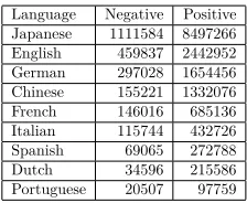
Language Negative Positive Japanese 1111584 8497266 English 459837 2442952 German 297028 1654456 Chinese 155221 1332076 French 146016 685136 Italian 115744 432726 Spanish 69065 272788 Dutch 34596 215586 Portuguese 20507 97759

Table 1: Number of negative and positive documents for each language in our data set

and TripAdvisor. The Portuguese data was mined from Walmart5_{, Opinaki}6_{, Buscap}_´_e7_, and TripAdvisor. The Dutch data was mined from bol.com8_{, Ciao!, and TripAdvisor. The} Chinese data was mined from Amazon, dangdang.com9_{, and TripAdvisor. The Japanese} data was mined from Amazon, Rakuten10_{, and Kakaku.com}11_{. Across these web sites,} these languages are not equally well-represented. As a consequence, for some of the lan-guages (e.g. Japanese) we were able to mine substantially more data than for others (e.g. Portuguese) (Table 1).

4 Document Representation

A text document is a sequence of tokens. Tokens can simply be single characters within the text document. However, in sentiment classiﬁcation, the tokens of interest are typically n-grams, which are n-length sequences of contiguous whitespace-separated words. For example, if a document is the sequence (W1,W2, . . . ,WN−1,WN), where

W2, . . . ,WN−1 are whitespace-separated words, andW1 and WN are the special symbol <BOUNDARY>, signifying the beginning or the end of the document, then the2-grams are (W1,W2),(W2,W3),(W3,W4), . . . ,(WN−2,WN−1),(WN−1,WN).

In Chinese and Japanese, words are not delimited by whitespace in writing. For the results we present in this paper, we used third-party libraries (Taketa, 2012; Lin, 2012) to segment Chinese and Japanese documents into words. These libraries are based on machine learning methods, and do not require large dictionary ﬁles. Nie et al. (Nie et al., 2000) considered tokenizing Chinese documents asn-grams. We also experimented with this approach for both Chinese and Japanese documents (i.e. we treated single characters as tokens). Al-though we do not present them here, the results we achieved in these experiments were comparable to (though not quite as good as) the results we achieved with the third-party libraries.

(5)

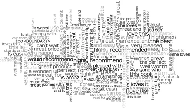
Figure 1: English2-grams most indicative of positive sentiment.

4.1 Generalized N-gram

We can generalize then-gram model by introducing a window sizek≥n. To iterate over all the tokens in a sequence, we ﬁrst consider every window in the sequence (that is, every contiguous subsequence of lengthk). The tokens are all the (not necessarily contiguous) subsequences of lengthnwithin each window. Whenk=n, this is just the standardn-gram model. Guthrie et al. (Guthrie et al., 2006) refer to this as the skip-gram model.

This model is suitable for languages with a flexible word order (e.g. German). With a flex-ible word order, the co-occurrence of several specific words in proximity may be indicative of a particular sentiment irrespective of any intermediary words. In the standardn-gram model, the relevant words can only be captured in a token along with the intermediary words. Due to the potential variety in the intermediary words, a single document may contain many tokens that are different, but that all correspond to the co-occurrence of these relevant words. In contrast, the generalized n-gram model enables these relevant words to be captured in a single token. This helps to mitigate against noise. However, for a given document, the generalizedn-gram model requires that more tokens are processed than does the standardn-gram model.

4.2 Hitting N-gram

(6)

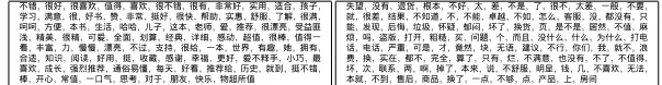
不错,很好,很喜欢,值得,喜欢,很不错,很有,非常好,实用,适合,孩子,

Table 2: Top Chinese automatically segmented words most indicative of positive and negative sentiment.

great, love, easy, highly, best, perfect, excellent, amazing, loves, wonderful, favorite, awesome, fantastic, recommend, book, beautiful, perfectly, pleased, sturdy, fits, works, rec-ommended, fun, definitely, life, price, album, comfortable, superb, happy, helps, gives, family, beautifully, brilliant, incredible, loved, classic, makes, glad, fast, delicious, out-standing, allows, easily, little, always, cd, heart, durable, easier, enjoy, unique, provides, truly, beat, favorites, solid, simple, handy, songs, collection, powerful, ease, size, super, greatest, keeps, song, smooth, books, thank, bonus, nicely, brings, friends, amazed, pleasantly, holds, terrific, gift, wonderfully, hooked, read, quick, enjoyed, skeptical, fabulous, thanks, compact, stores, favourite, al-bums, refreshing, learning, addictive, penny, guitar, gor-geous, sharp, journey, enjoys, lives, colors, joy, compli-ments, worry, job, versatile, must, every, informative, soft, everyone, daughter, comes, everyday, masterpiece, satisfied, crisp, affordable, fascinating

poor, bad, waste, worst, money, customer, return, dis-appointed, service, but, refund, told, terrible, returned, nothing, did, unfortunately, hotel, didn’t, back, horrible, worse, problem, sent, useless, ok, company, awful, disap-pointing, off, tried, why, stay, pay, asked, send, should, returning, do, disappointment, poorly, don’t, phone, bor-ing, again, staff, said, call, trybor-ing, support, guess, maybe, rude, unless, instead, get, seemed, supposed, contacted, paid, wouldn’t, fix, went, stopped, thought, avoid, beware, defective, customers, received, sorry, booked, <NUM-BER>, broke, manager, wrong, warranty, junk, mistake, wasted, rooms, contact, left, never, doesn’t, me, bro-ken, replacement, failed, happened, crap, email, stupid, garbage, annoying, wasn’t, least, star, cheap, reviews, months, properly, apparently, weeks, response, checked, working, got, frustrating, stayed, slow, going, hoping, waiting, error, ridiculous, completely, reason, try, either, credit, ended, please, half

Table 3: Top English words most indicative of positive and negative sentiment.

excellent, permet, plaisir, magnifique, livre, découvrir, bonheur, recommande, facile, parfait, très, merveille, su-perbe, excellente, petit, parfaitement, grâce, agréable, the, régal, of, indispensable, également, grands, petits, facilement, douce, doux, j’adore, délicieux, chansons, con-seille, rock, l’album, bémol, idéal, simple, vivement, pou-vez, voix, cd, parfaite, meilleur, douceur, n’hésitez, adoré, délice, enfants, rapide, couleurs, bonne, magnifiques, grande, famille, toutes, génial, titres, découvert, pratique, to, pourrez, parfum, belle, adore, must, and, incontourn-able, aime, recommander, sublime, beauté, superbes, pe-tite, guitare, ouvrage, différentes, mélange, trouverez, bi-jou, lait, complet, sucre, remarquable, recette, univers, chanson, sel, modération, déguster, super

pas, ne, rien, service, client, me, réponse, disant, mau-vaise, j’ai, je, commande, pire, clients, mauvais, demande, aucune, déception, payer, mois, remboursement, impos-sible, déconseille, téléphone, n’est, dit, qu’ils, sav, mail, été, suis, déc�ue, mal, n’a, bref, bout, arnaque, deman-dé, n’ai, envoyé, eux, décevant, éviter, eu, n’y, prob-lème, commandé, semaines, rec�u, aucun, site, rembourser, payé, compte, personne, tard, contrat, chez, erreur, jours, n’était, mails, nul, courrier, déc�u, euros, responsable, là, aurait, avons, avoir, commercial, mon, rec�ois, médiocre, panne, désagréable, ma, sommes, vente, heureusement, chambre, c�a, colis, dû, j’avais, dommage, m’a, d’attente, j’appelle, semaine, retard, répond, n’ont, dossier, voulu, lendemain, pourtant, manque, étaient

Table 4: Top French words most indicative of positive and negative sentiment.

In contrast to the generalized n-gram model, the hitting n-gram model can drastically reduce the number of tokens that need to be processed, depending on the lexicon that is chosen. For this project, we processed our large data set using Pearson’s chi-squared test to ﬁnd the words that are most indicative of positive and negative sentiment to build a lexicon for each language. We discuss this in more detail in Section 5.

5 Classiﬁers

For our experiments, we modeled documents using the2-gram model, the generalized2 -gram model with window size 3, the generalized2-gram model with window size 5, and the hitting2-gram model with (preceding) window size 1. For each of these models, we trained a naive Bayes classifier and a logistic regression classifier. During testing, we considered the results from the naive Bayes classifier, and the naive Bayes classifier boosted with the logistic regression classifier using majority vote. We repeated this for each language.

5.1 Hitting

2 -gram Model

(7)

to be the most effective. We used Pearson’s chi-squared test to find, for each language, the top 200 words most indicative of positive sentiment and the top 200 words most indicative of negative sentiment, without filtering for stop words (e.g. Table 2, Table 3, and Table 4). We used these words as the lexicon for the hitting2-gram model.

Following Yang and Pedersen, we computed, for each wordw and each sentiments, the goodness of ﬁt measure:

χ2(w,s) = N×(AD−CB)

2

(A+C)×(B+D)×(A+B)×(C+D)

whereAis the number of documents with sentimentsin whichwoccurs,Bis the number of documents without sentimentsin whichwoccurs,C is the number of documents with sentimentsin whichwdoes not occur,Dis the number of documents without sentiments

in whichwdoes not occur, andNis the total number of documents. We did this once over our entire data set, and took the words that scored highest according to this measure.

In our experiments, we set the window size to be 1 preceding word. We also tried other window sizes, but they did not produce substantially better results. We do not report these other results.

The technique we used to build the lexicon can be applied to other kinds of tokens. For example, Figure 1 is a word cloud of the English 2-grams most indicative of positive sentiment in our data set. We generated the word cloud using Wordle (Feinberg, 2012).

5.2 Naive Bayes Classiﬁer

For the2-gram model, we used the training data to compute for each2-gram,(W,W0₎_{, the}

probability that it belongs to a document with a positive sentiment,Ppos(W,W0₎_{, and the}

probability that it belongs to a document with a negative sentiment,Pneg(W,W0₎_{. Given a}

document(W1,W2, . . . ,WN−1,WN)12to classify, we apply a decision rule based on the ratio ∏

i

Ppos(Wi,Wi−1)

Pneg(Wi,Wi−1)

computed using the probabilities determined from our training data. If this ratio is greater than1, then we classify the document as positive. Otherwise, we classify the document as negative.

The following derivation show what this ratio means. ∏

2, . . . ,WN−1are whitespace-separated words, andW1 andWN are the special symbol<BOUNDARY>,

(8)

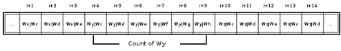
Figure 2: Sum over the range to get the count forWy.

Line(1)follows from the deﬁnition of conditional probability. Line(2)follows from com-mutativity and associativity of multiplication. Line (3)follows from the fact that the missing term

Ppos(WN)

Pneg(WN)=1

since the occurrence ofWN, the special symbol<BOUNDARY>, in a document with a posi-tive sentiment is equally likely to its occurrence in a document with a negaposi-tive sentiment. The numerator in the expression in line (3)is the probability that the given document has a positive sentiment according to both the2-gram model and the1-gram model. The denominator is the probability that the document has a negative sentiment according to both models. Our decision rule classifies the document according to which of these two probabilities is the greater. Notice that our confidence that the sentiment of the document was classified correctly can be increased using a threshold parameter. For example, if the ratio between the numerator and the denominator is very high, then we have high confi-dence that the document has a positive sentiment. At the cost of leaving some documents unclassified, the threshold parameter can be used to achieve arbitrarily high classification accuracies.

Our implementation allows these values to be computed quickly. We represent each distinct word that we encounter in the training data with a nonnegative32-bit integer, and use a hash map to store this representation. We represent each2-gram that we encounter in the training data by packing the two integers corresponding to the two words in the2 -gram in a64-bit integer. After processing the training data, we sort all the64-bit integers representing the2-grams, and store the sorted list in an array. We use the index of each

2-gram in this array as an index into two other arrays: one representing the number of occurrences of the2-grams in positive documents, and the other representing the number of occurrences of the2-grams in negative documents. This approach gives us a minimal perfect hash function from2-grams to their counts in positive and negative documents. Looking up a count for a given2-gram is fast: binary search on the sorted array gives us the index to the counts for occurrences in positive and negative documents. Our minimal use of pointers also keeps memory consumption low.

(9)

probability for a2-gram can be evaluated directly from this using Bayes’ rule.

The approach we took for the generalized2-gram models, and the hitting2-gram model is the same. However, the derivation for the value in our decision rule does not work out exactly, and only gives us a rough approximation of the probabilities. The results of the experiments reﬂect this fact: although classiﬁcation speed is very fast, the accuracies are somewhat less impressive than what one might expect.

5.3 Logistic Regression Classiﬁer

We used a logistic regression classifier provided by theLIBLINEARsoftware (Fan et al., 2008). For logistic regression, it is necessary to represent documents as feature vectors. We tried three representations. In all three cases, we had a feature for each token encountered in the training data. For the first representation, the value we used for each feature was the frequency of occurrence of the corresponding token, in the document. We normalized each feature to fall in the range[0, 1](details in the following paragraph). The second representation was like the first, except we normalized the whole vector to the unit vector, instead of normalizing per feature. For the third representation, the value we used for each feature was1or0, depending on whether the corresponding token was present in the document or not. We normalized the whole vector to the unit vector. All three approaches produced similar results. We only report the results for the first representation.

The normalization that we used for the ﬁrst representation is the following. Suppose_Dis the total set of training documents, andT is the total set of tokens encountered across all documents inD. For each documentd∈ Dand each tokent∈ T, letf reqd(t)be the frequency of occurrence of tokentin documentd(e.g. ifdcontains10tokens andtoccurs

5times ind, thenf reqd(t) =5/10=0.5). The normalized valuef req0

d(t)off reqd(t)is

f req0

d(t) =

f reqd(t)−mind0_∈D(f reqd0(t))

maxd0_∈D(f reqd0(t))−mind0_∈D(f reqd0(t)). Notice that ifdis a document from the testing set, thenf req0

d(t)can fall outside the range [0, 1]. This is the intended behavior (Fan et al., 2008; Hsu et al., 2010).

For our experiments, we boosted the naive Bayes classifier with the logistic regression classifier using majority vote. If both classifiers agreed, then we returned the value they agreed on. Otherwise, we returned no answer.

6 Experiments

6.1 Experimental Setup

For the empirical study, we evaluated two algorithms: a naive Bayes classifier, and a naive Bayes classifier boosted with a logistic regression classifier, using majority vote. In eval-uating each algorithm, we considered four ways of modeling text documents: the2-gram model (2g), the generalized2-gram model with window size 3 (2g-w3), the generalized

(10)

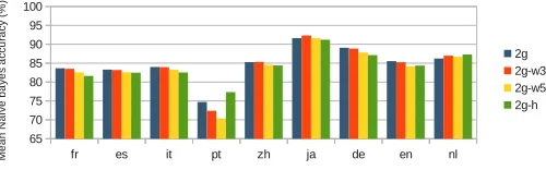
Figure 3: Mean accuracy (in percent, over ten runs) of naive Bayes classiﬁer for each model and each language.

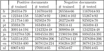
For each of the ten runs and each language, we sampled disjoint training and testing sets uniformly at random from the large data set. We ensured that the testing set was always at least four times larger than the training set. For each way of modeling text documents, we trained each algorithm using the training set, and tested it using the testing set. In Table 8, we report the mean and standard deviation, over ten runs, for the number of positive and negative documents in the training and testing sets for each language.

We performed our experiments using commodity hardware consisting of a quad-core Core 2 (Q9650) processor running at 3.0GHz, 16GB DDR2 memory running at 800MHz, and a 64-bit operating system with Linux kernel version 3.0. Our sentiment classiﬁcation system was implemented using Java, and we ran it using Oracle Java SE Runtime Environment (build 1.6.0 30-b12). Our system makes use of several third-party libraries. The versions of these that we used are JavaLIBLINEARversion 1.8 (Waldvogel, 2012), Apache Lucene Core version 3.6.0 (The Apache Software Foundation, 2012), cMeCab-Java version 2.0.1 (Taketa, 2012), and IK Analyzer 2012 upgrade 5 (Lin, 2012).

6.2 Results

Our multilingual sentiment classification system achieved very high accuracy (Table 6 and Table 7), without resorting to ad hoc NLP techniques, like parts-of-speech tagging and regular expression matching. It was also very fast (Table 5), because it did not rely on these techniques, which tend to be slow. The no answer rate for the naive Bayes classifier boosted with the logistic regression classifier is the rate at which documents were left unclassified because the two classifiers did not agree. Despite some documents being left unclassified, the two classifiers boosted together achieved a significantly higher accuracy than the naive Bayes classifier alone.

Recall from 5.2 that, in our implementation, the probability ratio in the decision rule of the naive Bayes classiﬁer is only a rough approximation of the true value for the generalized

2-gram model and the hitting2-gram model. The consequence of this is that we do not see a substantial improvement in classiﬁcation accuracy for these models (Figure 3).

(11)

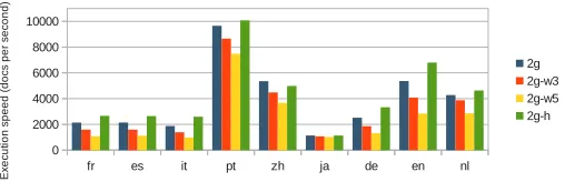
Figure 4: Mean classification speed (in documents per second per CPU core, over ten runs) of naive Bayes classifier boosted with logistic regression classifier for each model and each language.

Classiﬁcation speed (documents/second)

Table 5: Classification speed (mean and standard deviation, in documents per sec-ond, over ten runs) of naive Bayes classifier boosted with logistic regression classifier for each model and each language.

Table 6: Accuracy (mean and standard de-viation, in percent, over ten runs) of naive Bayes classiﬁer for each model and each language.

for Dutch is substantially greater than that for Portuguese. This is why the classification accuracy for Dutch did not suffer as much as it did for Portuguese. On the other hand, while the average testing document length for Chinese and Japanese is very short, we trained the algorithms with far more documents for these languages, and so the classification accuracies did not suffer. Thus, we can see a tradeoff between the amount of training data and the average length of the documents being classified. In our experiments with data from Twitter13_{(which we do not report in this paper), we found the same tradeoff: more} training data is needed to achieve higher classification accuracies with documents that are so short in length.

As expected, more unique tokens need to be processed during training as the window size for the generalized 2-gram model is increased (Table 9 and Figure 5). These are the unique tokens that are used to compute the probabilities, and construct the data structure discussed in 5.2. When the number of unique tokens encountered during training is greater, the amount of memory that is consumed during classiﬁcation is also greater. The classiﬁcation speed also decreases as the number of unique tokens increases. The hitting

2-gram model drastically reduces the number of unique tokens, and, unsurprisingly, has a faster classiﬁcation speed than the other models. The hitting2-gram model also achieves

(12)

Figure 5: Mean number of unique tokens after training (over ten runs) for each model and each language.

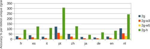
Figure 6: Mean accuracy per million unique tokens after training (in percent, over ten runs) of naive Bayes classiﬁer for each model and each language.

greater accuracy than the other models when the amount of training data is less (i.e. for Portuguese and Dutch). In Figure 6, we see that when we normalize for the number of unique tokens, the hitting2-gram model achieves far greater accuracy than the other models. Thus, for faster classiﬁcation speed, reduced memory consumption, and lower quality training data, the hitting2-gram is the way to go.

Our sentiment classification system was aggressively optimized for high speed and reduced memory consumption. The data for each language was aggregated in one flat file for ease of processing. Running the full set of ten runs of all experiments took less than an hour. Loading everything into memory consumed less than 3.5GB of the heap, which is unprecedented. When we ran the same set of experiments using LingPipe (Alias-i, 2012) for only the Spanish language and using only the2-gram model, we found that more than 12GB of heap memory were required to even finish training.

(13)

Accuracy No answer rate 2g 2g-w3 2g-w5 2g-h 2g 2g-w3 2g-w5 2g-h fr 91.3_±0.1 91.0_±0.1 90.6_±0.1 90.7_±0.1 14.2_±0.1 13.9_±0.1 14.1_±0.0 15.6_±0.1 es 90.4±0.1 90.3±0.1 90.1±0.1 89.8±0.1 14.5±0.1 14.5±0.2 14.7±0.2 14.2±0.2 it 91.7±0.1 91.6±0.1 91.3±0.1 91.1±0.1 14.9±0.1 14.8±0.2 15.1±0.2 15.5±0.1 pt 84.7±0.2 84.1±0.2 83.6±0.2 85.2±0.2 18.7±0.8 20.5±0.9 22.4±1.1 16.9±0.6 zh 91.0±0.0 90.8±0.1 90.3±0.0 90.6±0.1 11.7±0.1 11.2±0.1 11.0±0.1 12.3±0.1 ja 95.4_±0.0 95.5_±0.0 95.2_±0.0 95.1_±0.0 7.8_±0.1 7.2_±0.1 7.3_±0.1 7.7_±0.1 de 94.1_±0.0 93.8_±0.0 93.3_±0.0 93.5_±0.0 10.9_±0.1 10.6_±0.0 10.8_±0.1 12.1_±0.0 en 90.6±0.0 90.2±0.0 89.5±0.0 90.7±0.0 13.9±0.0 13.4±0.0 13.2±0.0 18.9±0.0 nl 92.0±0.1 91.7±0.1 91.0±0.1 91.7±0.2 17.1±0.2 15.3±0.1 14.3±0.1 16.2±0.2

Table 7: Accuracy and no answer rate (mean and standard deviation, in percent, over ten runs) of naive Bayes classiﬁer boosted with logistic regression classiﬁer for each model and each language.

Positive documents Negative documents # trained # tested # trained # tested fr 26455±79 116704±93 26556±66 116704±93 es 12234±158 55267±92 12061±102 55267±92 it 21175_±140 92502_±70 20272_±89 92502_±70 pt 3593±78 16349±43 2931±41 16349±43 zh 30914±194 124232±48 30989±48 124232±48 ja 218278±526 889453±391 219019±396 889453±391 de 54351±255 237839±206 54578±142 237839±206 en 87833_±400 367812_±224 85626_±207 367812_±224 nl 6907±83 27691±65 6765±67 27691±65

Table 8: Number of positive and negative documents in the training and testing sets (mean and standard deviation, over ten runs) for each language.

Number of unique tokens

2g 2g-w3 2g-w5 2g-h

fr 2914884±9360 6172487±20129 11914397±39474 882036±2352 es 2140713_±12048 4406273_±26340 8373245_±51332 664764_±3752 it 3425993±7458 7223768±16530 13926488±33039 749045±1400 pt 608836±1041 1165038±1953 2033085±3804 251139±499 zh 1640449±5753 3321802±11719 6219173±23299 667135±1756 ja 4142506±6055 10307368±14345 20572997±26398 2140987±2610 de 5372769±14153 10754868±29605 20217297±56647 1306724±2862 en 3290897±3804 6713768±7239 12604478±13434 1021480±1497 nl 809873_±2663 1508605_±5762 2634343_±11110 359049_±1642

Table 9: Number of unique tokens after training (mean and standard deviation, over ten runs) for each model and each language.

Conclusion and Future Work

In this paper, we presented an empirical study of two sentiment classification algorithms applied to nine languages (including Germanic, Romance, and East Asian languages). One of these algorithms is a naive Bayes classifier, and the other is an algorithm that boosts a naive Bayes classifier with a logistic regression classifier, using majority vote. We implemented these algorithms as part of a system for classifying the sentiment of multilingual text data. Our implementation is fast, and has high classification accuracy.

(14)

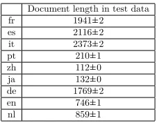
Document length in test data fr 1941±2 es 2116±2 it 2373_±2 pt 210±1 zh 112±0 ja 132±0 de 1769_±2 en 746±1 nl 859±1

Table 10: Mean document length, with standard deviation, over ten runs, in test data.

a variant of this generalization that helps reduce memory consumption. Along with the standardn-gram model, these two models are built into our system. We evaluated all of these models in the empirical study that we presented in this paper.

For the empirical study, we trained and tested our system on a data set that is substantially larger than that typically encountered in the literature. We generated this data set by crawling and mining various web sites for reviews of products and services. For each experiment in the study, we sampled disjoint training and testing sets uniformly at random from this large data set. Unlike the usual approach in the literature, the testing sets were much larger than the training sets (at least four times larger), and the experiments were repeated many times. We did this to ensure that our results were statistically signiﬁcant.

As we have shown in this paper, statistical methods applied to large amounts of data are effective for the sentiment classification problem. It would be interesting to investigate the application of this approach to the problem of relevance (i.e. determining whether a document conveys any sentiment at all). Previous efforts have been overly complicated (Pang and Lee, 2004). One approach that we are considering is to take a list ofn-grams that are most indicative of sentiment (determined using Pearson’s chi-squared test, as discussed in 5.1), and computing the mean and standard deviation for the frequency of occurrence of these words in the training documents. During testing, the frequency of occurrence for these words in the test documents can be compared to the mean we computed. If the frequency of occurrence is not less than one standard deviation below the mean, then a document can be deemed relevant.

We are also interested in commercializing our sentiment classification system by selling it to social media analytics firms, such as Sysomos14_{and BrandWatch}15_{. The existing} players in the sentiment classification field (e.g. Saplo16_{, Lexalytics}17_{, OpenAmplify}18_, and SNTMNT19_{) are not transparent about what they are doing, and it is not clear how} robust their offerings are. If commercialization fails, then we intend to make our sentiment classification system freely available under the GPL20_{, since one of our great passions is} educating the public on the power of machine learning methods.

14_{http://www.sysomos.com} 15_{http://www.brandwatch.com} 16_{http://saplo.com}

17_{http://www.lexalytics.com} 18_{http://www.openamplify.com} 19_{http://www.sntmnt.com}

(15)

References

Alias-i (2012). Lingpipe version 4.1.0.http://alias-i.com/lingpipe/index.html.

The Apache Software Foundation (2012). Apache Lucene Core version 3.6.0. http: //lucene.apache.org/core.

Bengio, Y., Ducharme, R., Vincent, P., and Janvin, C. (2003). A neural probabilistic language model.The Journal of Machine Learning Research, 3(Feb):1137–1155.

Bespalov, D., Bai, B., Qi, Y., and Shokoufandeh, A. (2011). Sentiment classiﬁcation based on supervised latent n-gram analysis. InProceedings of the 20th ACM International Conference on Information and Knowledge Management (CIKM ’11), pages 375–382.

Chang, C.-C. and Lin, C.-J. (2011). LIBSVM: A library for support vector machines. ACM Transactions on Intelligent Systems and Technology, 2(3):27:1–27:27. Software available athttp://www.csie.ntu.edu.tw/~cjlin/libsvm.

Collobert, R. and Weston, J. (2008). A uniﬁed architecture for natural language process-ing: deep neural networks with multitask learning. InProceedings of the 25th International Conference on Machine Learning (ICML ’08), pages 160–167.

Cormen, T. H., Leiserson, C. E., Rivest, R. L., and Stein, C. (2001). Introduction to Algorithms. MIT Press and McGraw-Hill, 2nd edition.

Cortes, C. and Vapnik, V. (1995). Support-vector networks. Machine Learning, 20(3): 273–297.

Csisz´ar, I. (1996). Maxent, mathematics, and information theory. In Hanson, K. M. and Silver, R. N., editors,Maximum Entropy and Bayesian Methods: Proceedings of the 15th International Workshop on Maximum Entropy and Bayesian Methods, pages 35–50.

Domingos, P. and Pazzani, M. (1997). On the optimality of the simple bayesian classi-ﬁer under zero-one loss. Machine Learning - Special issue on learning with probabilistic representations, 29(2-3):103–130.

Fan, R.-E., Chang, K.-W., Hsieh, C.-J., Wang, X.-R., and Lin, C.-J. (2008). LIBLIN-EAR: A library for large linear classiﬁcation. The Journal of Machine Learning Re-search, 9(Aug):1871–1874. Software available athttp://www.csie.ntu.edu.tw/~cjlin/ liblinear.

Feinberg, J. (2012). Wordle.http://www.wordle.net/.

Guthrie, D., Allison, B., Liu, W., Guthrie, L., and Wilks, Y. (2006). A closer look at skip-gram modelling. InProceedings of the Fifth International Conference on Language Resources and Evaluation (LREC–2006), pages 1222–1225.

Hsu, C.-W., Chang, C.-C., and Lin, C.-J. (2010). A practical guide to support vector classication.http://www.csie.ntu.edu.tw/~cjlin/papers/guide/guide.pdf.

(16)

Joachims, T. (1999). Making large-scale support vector machine learning practical. In Sch¨olkopf, B. and Smola, A., editors,Advances in kernel methods, pages 169–184. MIT Press Cambridge, MA, USA.

Lewis, D. D. (1998). Naive (bayes) at forty: The independence assumption in information retrieval. InProceedings of the 10th European Conference on Machine Learning (ECML ’98), pages 4–15.

Lin, L. Y. (2012). IK Analyzer 2012 upgrade 5. http://code.google.com/p/ ik-analyzer.

Nie, J.-Y., Gao, J., Zhang, J., and Zhou, M. (2000). On the use of words and n-grams for chinese information retrieval. InProceedings of the Fifth International Workshop on Information Retrieval with Asian Languages (IRAL ’00), pages 141–148.

Nigam, K., Laﬀerty, J., and McCallum, A. (1999). Using maximum entropy for text classiﬁcation. InWorkshop on Machine Learning for Information Filtering (IJCAI ’99), pages 61–67.

Pang, B. and Lee, L. (2004). A sentimental education: sentiment analysis using subjec-tivity summarization based on minimum cuts. InProceedings of the 42nd Annual Meeting on Association for Computational Linguistics (ACL ’04).

Pang, B. and Lee, L. (2008). Opinion mining and sentiment analysis. Foundations and Trends in Information Retrieval, 2(1-2):1–135.

Pang, B., Lee, L., and Vaithyanathan, S. (2002). Thumbs up?: sentiment classiﬁcation using machine learning techniques. InProceedings of the ACL-02 conference on Empirical methods in natural language processing (EMNLP ’02), pages 79–86.

Rosenblatt, F. (1957). The perceptron–a perceiving and recognizing automaton. Technical Report 85-460-1, Cornell Aeronautical Laboratory.

Taketa, K. (2012). cMeCab-Java version 2.0.1. http://code.google.com/p/ cmecab-java.

Waldvogel, B. (2012). Java LIBLINEAR version 1.8. http://www.bwaldvogel.de/ liblinear-java/.