Coarse-Grid Computational Fluid Dynamics (CG-CFD) Error Prediction using Machine Learning.

(1)

ABSTRACT

HANNA, BOTROS NASEIF HANNA BISHARA. Coarse-Grid Computational Fluid Dynamics (CG-CFD) Error Prediction using Machine Learning. (Under the direction of Dr. Nam T. Dinh and Dr. Igor A. Bolotnov).

Nuclear reactor safety research requires analysis of a broad range of accident scenarios.

One of the major safety barriers against nuclear fission products release is the containment

structure. Modeling and simulation are essential tools to identify parameters affecting Containment

Thermal Hydraulics (CTH) phenomena. The thermal-hydraulic modeling approaches used in the

nuclear industry can be classified into two categories: system-level codes and Computational Fluid

Dynamics (CFD) codes. System codes are not as capable as CFD of capturing and giving detailed

knowledge of the multi-dimensional behavior of CTH phenomena. However, CFD computational

cost is high when modeling complex accident scenarios, especially the ones which involve

longtime transients. The high expense of traditional CFD is due to the need for computational grid

refinement to guarantee that the solutions are grid independent.

To mitigate the computational expense, it is proposed to rely on coarse-grid CFD

(CG-CFD). Coarsening the computational grid makes the computation significantly more affordable for

practical applications, but it also increases the discretization (grid-induced) error which depends

on the grid size and varies with space and time. Hence, a method is developed to produce a

surrogate model, that predicts the distribution of the CG-CFD local error, to correct the flow

variables of interest. Given high-fidelity simulations (sufficiently fine-mesh simulations), a

surrogate model is trained to predict the CG-CFD local errors as a function of the coarse-grid local

flow features. The surrogate model is constructed using machine learning regression algorithms

(2)

This proposed method is applied to a three-dimensional turbulent flow inside a lid-driven

cavity domain. A set of scenarios that test the proposed method are studied. These scenarios

investigate the capability of the surrogate model to interpolate and extrapolate outside the training

data range. These scenarios also cover a range of Reynolds number in the turbulent flow and

transitional flow range plus a range of grid sizes, aspect ratios and different variables of interest.

Based on the investigated cases: it was found that the random forest regression technique is

predicting the grid-induced error better than the neural network although random forest technique

is computationally cheaper. The proposed method maximizes the benefit of the available data and

shows a potential for a good predictive capability.

The proposed CG-CFD approach is different from conventional CFD for two reasons: (1)

Typically, for each new fluid flow problem, a new simulation is needed, and a grid-independent

solution is required, even if the new flow problem is only slightly different from old one. In the

proposed CG-CFD method, the available data are utilized to predict the variable of interest for the

new flow problem (that is simulated by a coarse grid) given the available high-fidelity data. The

success of this approach is based on the assumption that the available high-fidelity data and the

new flow problem have similar physics. (2) In conventional turbulence modeling, turbulence

models typically rely on incorporating more physics and using empirical models for some

parameters based on the available validation data. For different flow conditions, new turbulence

models may be constructed. The proposed method is data driven so each new experimental data or

(3)

(4)

Coarse-Grid Computational Fluid Dynamics (CG-CFD) Error Prediction using Machine Learning.

by

Botros Naseif Hanna Bishara Hanna

A dissertation submitted to the Graduate Faculty of North Carolina State University

in partial fulfillment of the requirements for the degree of

Doctor of Philosophy

Nuclear Engineering

Raleigh, North Carolina

2018

APPROVED BY:

_______________________________ _______________________________ Dr. Nam T. Dinh Dr. Igor A. Bolotnov

Committee Co-Chair Committee Co-Chair

(5)

ii DEDICATION

To my Father, Mikhaeel Hanna Who always supported me.

(6)

iii BIOGRAPHY

The author, Botros N. Hanna was born in March 1988 in Athribis in lower Egypt. His given

name (Botros) means the stone. He is the first child of his father, Mikhaeel Hanna and his mother,

Sonia Samaan. He has one younger brother (Pemen). Botros was married to Monika Attia in

January 2016.

Botros earned the bachelor’s degree in Nuclear Engineering with a degree of honors from

Alexandria University in 2010. In Fall 2012, Botros joined the Department of Nuclear Engineering

in North Carolina State University as a graduate student. He started his graduate studies with Dr.

Igor A. Bolotnov and Dr. Nam T. Dinh in Fall 2013 to get his Master of Science degree in 2015.

His research areas include computational fluid dynamics for nuclear engineering applications plus

application of machine learning algorithms to develop big-data-driven physics-informed models.

He successfully defended his PhD dissertation in April 2018.

(7)

iv ACKNOWLEDGMENTS

I give my ultimate thanks to God who has given me the power and persistence to get where

I am today. I cannot thank enough my beloved spouse, Monika who has been my beautiful wife,

life companion and stayed by my side in good and hard times. I am incredibly thankful for my

family; my mother who always believed in me, my father for his limitless love and support and

my brother who is always the best friend. I also acknowledge the guidance of those who

encouraged me to pursue my studies in USA (Dr. Hanaa Abou Gabal and Dr. Alya Badawi in

Alexandria University, Egypt).

I would like to express my gratitude to Dr. Igor A. Bolotnov and Dr. Nam T. Dinh for their

consistent support throughout my Ph.D. journey. They always provided me with their insightful

discussions about the research. They encouraged me to be an independent researcher and they were

always great examples to follow in academic research. I also acknowledge the advice and

recommendations by Dr. Robert Youngblood and Dr. Tiegang Fang.

I also acknowledge the support of the Idaho National Laboratory through its National

University Consortium and Laboratory Directed Research & Development (LDRD) Program

under DOE Idaho Operations Office and the Nuclear Engineering Department at NC State

University.

(8)

v TABLE OF CONTENTS

LIST OF TABLES ... viii

LIST OF FIGURES ... ix

ABBREVIATIONS ... xii

NOMENCLATURE ... xiv

1. INTRODUCTION ... 1

1.1. Objectives ... 2

1.2. An Overview of System Codes for Nuclear Thermal Hydraulics ... 2

1.3. An Overview of CFD Codes for Nuclear Thermal Hydraulics ... 4

1.4. Motivation: The Need for Data-Driven Models ... 5

1.5. Progress in Data-Driven Models in Fluid Dynamics ... 6

1.5.1. Autonomic sub-grid Large Eddy Simulation (ALES) ... 6

1.5.2. Autonomic sub- Closure Term in a Bubbly Flow Equation ... 7

1.5.3. RANS Model Discrepancy ... 8

1.5.4. Smoothed Particle Hydrodynamics... 11

1.6. CG-CFD for Simulating CTH ... 11

1.7. The Scope of This Work ... 14

1.7.1. Present Approach vs. Traditional CFD ... 15

1.7.2. Present Research vs. Turbulence Modeling Error Reduction ... 16

1.7.3. This Work vs. Reduced Order Modeling (ROM) ... 17

1.8. The Structure of This Dissertation ... 18

1.9. Definitions ... 18

1.10. Chapter Summary ... 19

2. TURBULENCE MODELING ... 21

2.2. Basics of the Turbulence Theory ... 21

2.3. Large Eddy Simulation (LES) ... 23

2.4. Reynolds Averaged Navier-Stokes (RANS) Equations ... 27

2.5. Grid-Induced Error in LES, RANS, and CG-CFD ... 30

2.5.1. LES ... 30

2.5.2. RANS ... 31

(9)

vi

3. NUMERICAL SOLUTION ERROR ... 34

3.2. Discretization Methods ... 34

3.2.1. Finite Difference Method (FDM) ... 35

3.2.2. Finite Element Method (FEM) ... 36

3.2.3. Finite Volume Method (FVM) ... 37

3.3. Iterative Methods... 40

3.4. Discretization Error ... 41

3.5. Iterative Convergence Error ... 42

4. MACHINE LEARNING ... 45

4.2. Clustering ... 47

4.3. Dimensionality Reduction ... 48

4.4. Classification ... 49

4.5. Regression ... 51

4.5.1. Artificial Neural Network (ANN) ... 51

4.5.2. Deep Learning ... 54

4.5.3. Random Forest Regression ... 55

5. COARSE-GRID ERROR PREDICTION METHOD ... 59

5.2. Problem Statement ... 59

5.3. Research Hypothesis ... 60

5.4. Proposed Approach ... 62

5.4.1. CG-CFD Error Prediction Method ... 62

5.4.2. Features Selection ... 64

5.4.3. Data Comparison (Mapping) ... 65

5.4.4. Data Normalization ... 66

5.4.5. Machine Learning Error Assessment... 67

5.5. Case Study ... 68

5.5.1. Numerical Simulations ... 69

(10)

vii

5.6. Summary ... 73

6. RESULTS AND DISCUSSIONS ... 74

6.2. Validation ... 74

6.3. Training and Testing Cases ... 75

6.3.1. Scenario I: Reynolds Number Interpolation ... 77

6.3.2. Scenarios II and III: Reynolds Number Extrapolation. ... 81

6.3.3. Scenarios IV, V and VI: Grid Size Interpolation and Extrapolation. ... 91

6.3.4. Scenarios VII, VIII and IX: Reynolds Number and Grid Size Interpolation and Extrapolation. ... 91

6.3.5. Other Variables 𝑈𝑦 and 𝑈𝑧 ... 91

6.3.6. Computational Time for Big Data ... 98

6.3.7. Data Convergence ... 98

6.3.8. Scenario X: Different grid spacing in different directions. ... 104

6.3.9. Scenario XI, XII and XIII (Extrapolation to Aspect Ratio =1.2). ... 105

6.3.10. Scenario XIV, XV, XVI, XVII and XVIII (Aspect Ratio Interpolation and Extrapolation up to Aspect Ratio = 4). ... 105

7. CONCLUSIONS... 121

7.1. Contributions ... 121

7.2. Future Work ... 123

(11)

viii LIST OF TABLES

Table 1 A Comparison between two approaches for data-driven turbulence modeling. ... 9

Table 2 Different RANS turbulence models ... 29

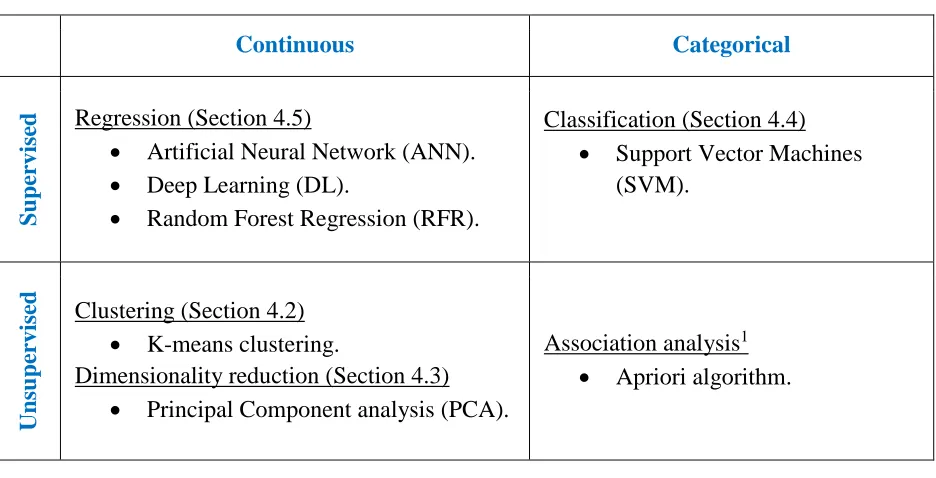
Table 3 Taxonomy of ML algorithms. ... 46

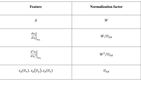
Table 4 Normalization factors for different variables.s ... 67

Table 5 Training and testing data (first set of scenarios in terms of Re and ∆). Re and Δ are the Reynolds number and the grid spacing, respectively. ... 71

Table 6 Training and testing data (second set of scenarios in terms of 𝑅𝑒, ∆, and 𝐻/𝑊). 𝑅𝑒, 𝛥, and 𝐻/𝑊 are the Reynolds number, grid spacing and aspect ratio,respectively ... 72

Table 7 A comparison between different scenarios in terms of ML error and computational time. ... 86

Table 8 Data convergence study. ... 104

(12)

ix LIST OF FIGURES

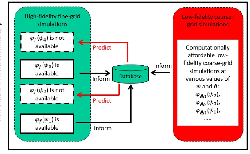
Figure 1 A conceptual framework for simulating CTH with CG-CFD. The focus of

this work is highlighted in yellow. ... 12

Figure 2 A snapshot of the velocity (𝑈𝑦) profile in a three-dimensional quasi- steady state turbulent flow in a lid-driven cavity. The lid is moving in 𝑥- direction. The profile is computed with a fine grid (left) and a coarse- grid (right). The fine-grid result is mapped to a coarse-grid (in the middle). ... 13

Figure 3 CFD sources of error. ... 15

Figure 4 Distribution of turbulent energy in wavenumber space. ... 22

Figure 5 Computational expense (of DNS, LES, and RANS) as a function of Reynolds number. ... 27

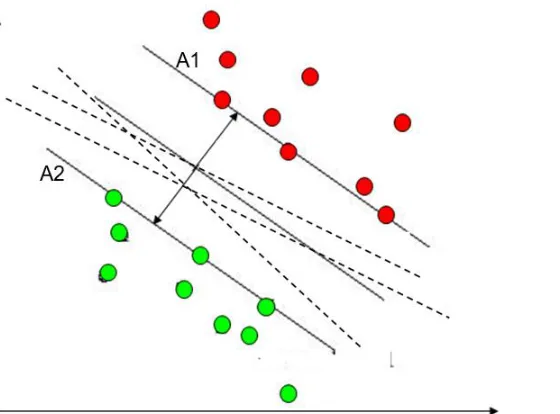
Figure 6 Illustration of the classification problem: various dashed lines separating two groups of data. ... 50

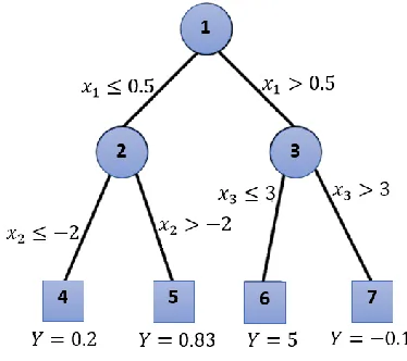
Figure 7 Regression tree. ... 56

Figure 8 Workflow for data generation in the CG-CFD problem. ... 60

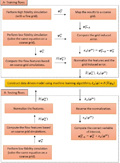
Figure 9 The proposed method to predict CG-CFD error using ML algorithms. ... 63

Figure 10 Mapping flow variable, computed by a fine grid onto a coarse grid by one of two approaches: point to point (top) or cell to cell (bottom). ... 66

Figure 11 Lid-driven cubic cavity. The lid velocity is parallel to the 𝑥-axis. ... 69

Figure 12 The axial profile (𝑦 direction) for velocity, 𝑈𝑥 (top) and the axial profile (𝑥 direction for the velocity, 𝑈𝑦 (bottom) at 𝑅𝑒 = 12000. ... 76

Figure 13 A representation of one-hidden-layer ANN with 37 inputs, 20 neurons and one output as represented by MATLAB [25]. 𝑤 and 𝑏 represent the weights and biases as presented in Section 4.5.1. ... 77

Figure 14 ANN performance in scenario I (training flows). MSE vs. the number of iterations (epochs) (above). 𝜀𝛥𝑈𝑥 expected by ANN vs. the actual 𝜀𝛥𝑈𝑥 (below). ... 78

Figure 15 Scenario I (Reynolds number interpolation) for 𝑈𝑥 (by ANN). ∆= 0.033𝑚. Training data (above) and testing data (below). CG: Coarse grid predictions. ML: Machine learning predictions. ... 80

Figure 16 RFR OOB error decreases with increasing number of trees. ... 82

(13)

x Figure 18 Scenario II (Reynolds number extrapolation to a higher value) for 𝑈𝑥 (by

ANN). ∆= 0.033𝑚. Training data (above) and testing data (below). ... 84

Figure 19 Scenario II (Reynolds number extrapolation to a higher value) for 𝑈𝑥 (by

RFR). ∆= 0.033𝑚. Training data (above) and testing data (below). ... 85

Figure 20 A representation of Three-hidden-layer ANN with 37 inputs, 20 neurons

for each layer and one output as represented by MATLAB [25]. ... 87

Figure 21 Effect of increasing the number of neural network layers on ML error for

the scenario I (above) and the scenario II (below). ... 88

Figure 22 Effect of increasing the number of neural network layers on the

computational time. ... 89

Figure 23 Scenario III (Reynolds number extrapolation to a lower value) for 𝑈𝑥 (by

RFR). ∆= 0.033𝑚. Training data (above) and testing data (below). ... 90

Figure 24 Scenario IV (grid size interpolation) for 𝑈𝑥 (by RFR). 𝑅𝑒 = 12000.

Training data (above) and testing data (below). ... 92

Figure 25 Scenario V (grid size extrapolation to a finer grid) for 𝑈𝑥 (by RFR).

𝑅𝑒 = 12000. Training data (above) and testing data (below). ... 93

Figure 26 Scenario VI (grid size extrapolation to a coarser grid) for 𝑈𝑥 (by RFR).

𝑅𝑒 = 12000. Training data (above) and testing data (below). ... 94

Figure 27 Scenario VII (Reynolds number and grid size interpolation) for 𝑈𝑥 (by

RFR). Training data (above) and testing data (below). ... 95

Figure 28 Scenario VIII (extrapolation to a higher Reynolds number and a finer grid)

for 𝑈𝑥 (by RFR). Training data (above) and testing data (below). ... 96

Figure 29 Scenario IX (extrapolation to a lower Reynolds number and a coarser grid)

Figure 30 Scenario VII (Reynolds number and grid size interpolation) for 𝑈𝑦 (by RFR).

Figure 31 Scenario VIII (extrapolation to a higher Reynolds number and a finer grid)

𝑈𝑦 (by RFR). Training data (above) and testing data (below). ... 100

Figure 32 Scenario VII (Reynolds number and grid size interpolation) for 𝑈𝑧 (by RFR).

Figure 33 Scenario VIII (extrapolation to a higher Reynolds number and a finer grid) for

𝑈𝑧 (by RFR). Training data (above) and testing data (below). ... 102

Figure 34 Big-data computational cost using random forest regression. ... 103

Figure 35 Scenario X (different grid spacing in different directions) for 𝑈𝑥 (by RFR).

(14)

xi Figure 36 Scenario XI (aspect ratio extrapolation) for 𝑈𝑥 (by RFR). Training data

(above) and testing data (below). ... 107

Figure 37 Scenario XII (aspect ratio and Reynolds number extrapolation) for 𝑈𝑥

(by RFR). Training data (above) and testing data (below). ... 108

Figure 38 Scenario XIII (aspect ratio, Reynolds number, and grid size extrapolation)

Figure 39 Scenario XIV (aspect ratio interpolation) for Ux (by RFR). Training data

(above) and testing data (below). ... 111

Figure 40 Scenario XIV (aspect ratio interpolation), after adding new features, for 𝑈𝑥

(by RFR) Training data (above) and testing data (below). ... 112

Figure 41 Scenario XV (aspect ratio extrapolation to a lower ratio), for 𝑈𝑥 (by RFR).

Figure 42 Scenario XVI (aspect ratio extrapolation to a higher ratio), for 𝑈𝑥 (by RFR).

Figure 43 Velocity profile in x-direction inside the lid-driven cavity flow for different

aspect ratios at 𝑅𝑒 = 6000. ... 115

Figure 44 Training data from different aspect ratios and grid sizes for scenario XVII

and XVIII for 𝑈𝑥 (by RFR) at 𝑅𝑒 = 12000. ... 116

Figure 45 Testing data for scenario XVII (aspect ratio extrapolation) for 𝑈𝑥 (by RFR)

at 𝑅𝑒 = 12000. ... 117

Figure 46 Testing data for scenario XVIII (aspect ratio and grid size extrapolation) for

𝑈𝑥 (by RFR) at 𝑅𝑒 = 12000. ... 117

Figure 47 Velocity profile in 𝑥 direction inside the lid-driven cavity flow for different

(15)

xii ABBREVIATIONS

ALES Autonomic sub-grid Large Eddy Simulation

ANN Artificial Neural Network

BD Blended Difference

BWR Boiling Water Reactor

CD Central Difference

CFD Computational Fluid Dynamics

CG Coarse Grid

CG-CFD Coarse-Grid Computational Fluid Dynamics

CTH Containment Thermal Hydraulics

DL Deep Learning

DNS Direct Numerical Simulation

FDM Finite Difference Method

FEM Finite Element Method

FVM Finite Volume Method

HF High Fidelity

KDE Kernel Density Estimation

LES Large Eddy Simulation

LF Low Fidelity

MATLAB Matrix Laboratory

MD Mahalanobis Distance

ML Machine Learning

(16)

xiii

NPP Nuclear Power Plant

NS Navier – Stokes

OOB Out Of Bag

OpenFOAM Open source Field Operation And Manipulation

PC Principal Component

PCA Principal Component Analysis

PDE Partial Differential Equation

PIML Physics Informed Machine Learning

PISO Pressure Implicit Splitting of Operators

QOI Quantity Of Interest

RANS Reynolds Averaged Navier-Stokes

RFR Random Forest Regression

RISMC Risk-Informed Safety Margin Characterization

ROM Reduced Order Modeling

SGS Sub-Grid Scale

SVM Support Vector Machines

TE Truncation Error

TH Thermal Hydraulics

TKE Turbulence Kinetic Energy

(17)

xiv NOMENCLATURE

𝐶𝑠 Smagorinsky constant

𝐸(𝜅_𝑙) The energy contained in the eddies of size 𝑙 𝐸_𝑀𝑙 Machine learning algorithm error

𝐹 Surrogate function

𝐻/𝑊 The aspect ratio (height to width ratio)

𝐿 Discrete operator

𝐿𝑓 Discrete operator computed by a fine grid

𝐿𝑠 The mixing length for sub-grid scales

𝐿𝛥 Discrete operator computed by a grid, 𝛥

𝑃 The rate of turbulence energy production

𝑄 The second invariant of the velocity gradient tensor

𝑅 Correlation coefficient

𝑅𝑒 Reynolds number

𝑅𝑒_𝜏 Wall-shear stress-based Reynolds numbers

𝑅𝑒𝑡 Turbulent Reynolds number

𝑅𝑒∆ Cell Reynolds number

𝑆𝑖 Silhouette value

T Target

𝑼 Velocity vector

(18)

xv

𝑉 Volume

W Cavity width (or cavity lid width)

X Features (inputs) in machine learning algorithm

𝑋̃ Normalized features

𝑌+ _𝑌+ ₌ 𝑢∗𝑑

ν , dimensionless wall distance

𝑑 Distance to the nearest wall

𝑘 Turbulent kinetic energy

𝑙 Length scale

𝑙𝑚 Mixing length

𝑛 Control volume surface normal

𝑝𝑘 Kinematic pressure

𝑡 Time

𝑢_∗ Friction velocity at the nearest wall x, y, z Cartesian coordinates

Greek letters

∆ Grid spacing or cell length

∆𝑥, ∆𝑦, ∆𝑧 Grid spacing in the three Cartesian directions: x, y, z

𝛿𝑖𝑗 Kronecker delta

𝜀 The rate of dissipation of the turbulence kinetic energy

(19)

xvi

𝜀̃_𝛥 Normalized grid-induced error

𝜂 Kolmogorov length scale

𝜅_𝑙 The wavenumber of an eddy of size is 𝑙

𝜈 Kinematic viscosity

𝜈𝑠𝑔𝑠 Sub-grid scale viscosity

𝜈𝑡 Turbulent kinematic viscosity

𝜈̃𝑡 Spalart-Allmaras model variable (viscosity like variable)

𝜎 Standard deviation

𝜏 Reynolds stress

𝜏_𝑖𝑗

̅̅̅ Sub-grid scale stress tensor

𝜏_𝜂 Kolmogorov time scale

𝜑 Flow variable

𝜑̅ Filtered variable

𝜑_𝒄 Variable computed by a coarse-grid

𝜑_𝒇 Variable computed by a fine grid

𝜑_𝑓→𝛥 Flow variable computed by a fine grid and mapped onto a coarse-grid ∆ 𝜑𝑡𝑟 _{Flow variable distribution corresponding to the training data}

𝜑𝑡𝑒 _{Flow variable distribution corresponding to the testing data}

𝜑_𝛥 Flow variable computed by a grid, 𝛥

(20)

1

1. INTRODUCTION

Nuclear reactor safety analysis has received more attention since the Fukushima Daiichi

accident in 2011. Safety and design of Nuclear Power Plants (NPPs) imply studying Thermal

Hydraulics (TH) phenomena that may evolve during normal operation, design-basis accidents (that

NPP is designed to withstand) or severe accidents (that involve core melting) [1]. If an accident

occurs, the role of the reactor containment is vital as the major and final safety barrier. Hence,

predicting the Containment Thermal Hydraulics (CTH) phenomena impacts is needed to maintain

the integrity of the containment. Experiments that mimic the potential CTH phenomena are

necessary, but it is almost impossible to gain experimental full-scale data the cover all CTH

phenomena. Hence, for a complex system such as NPP, modeling and simulation are necessary

for performing safety analysis. There are various codes that are used to achieve this purpose: the

system TH codes (see Section 1.2) and Computational Fluid Dynamics (CFD) codes (see Section

1.3).

The system TH codes can model the entire reactor and its components as they include

multiple physics (fluid flow, heat transfer, neutron diffusion equations, etc.). However, system

codes have some limitations as they cannot capture the local three-dimensional complex

phenomena and they rely on many empirical correlations and parameters that are required due to

the lack of full understanding of the complex governing physics. Hence, CFD codes are needed to

capture the multi-dimensional behavior of the phenomena of interest. However, CFD approach is

computationally expensive for simulating complex systems with large computational domains.

The high expense of traditional CFD is due to the need for computational grid refinement to

guarantee that the solutions are grid-independent. To reduce the CFD computational cost, there is

(21)

2 It is proposed that the numerical error, which arises because of the coarse grids, can be

reduced/recovered using data-driven models. The need of data-driven CFD models, which benefit

from the available experimental and high-fidelity simulations, is emphasized in Section 1.4.

Currently, there is an increasing attention to the necessity of data-driven fluid dynamics’ models

that can be less expensive and more adaptable to the data (see Section 1.5).

This work proposes a framework to use a data-driven CG-CFD method in CTH field

(described in Section 1.6). To clarify the difference between the proposed data-driven CG-CFD

method and other approaches that aim to mitigate the complexity of CFD, the scope of this work

is presented in Section 1.7. Finally, the structure of the rest of the dissertation is described in

Section 1.8.

1.1.Objectives

The objectives of this chapter can be summarized as follows:

• Evaluating the capabilities and limitation of potential codes in CTH fields (system codes and

CFD).

• Introducing the motivation behind this research.

• Discussing the current research in data-driven CFD modeling.

• Developing a general framework to use CG-CFD simulations in CTH field.

1.2.An Overview of System Codes for Nuclear Thermal Hydraulics

System codes are designed to simulate the phenomena that are involved in design basis and

severe accidents. These codes utilize control volume approach to perform affordable computations.

Large control volumes are used to perform economic simulations. For instance, control volumes,

that are bigger than a one-meter cube, are used in phenomena-dominating regions (reactor vessel

(22)

3 bigger in other less-important regions in the nuclear system [2, 3]. Within each volume, time and

space dependent conservation equations for mass, momentum, and energy are solved for a

homogenous two-phase (steam-water) mixture. Phenomena are modeled with different degrees of

dimensionality [2]. Zero-dimensional (lumped parameter) models are used where the velocities

are low (e.g. reactor lower plenum). One-dimensional models are used where the flow has a

uniform direction (e.g. pipe flow). Three-dimensional models were developed for the components

with three-dimensional velocity (e.g. pressure vessel) with a coarse grid. Examples of system

codes include RELAP5 [3], MELCOR [4] and GOTHIC [5].

System codes are recognized in the nuclear industry as useful tools for analyzing accidents

and transients on the reactor system level. They represent the currently available knowledge and

can predict the figure of merit with computationally affordable simulations. However, system

codes still have some limitations. Among these limitations is the coarse-space resolution so the

small-scale phenomena are not resolved; Simulating highly turbulent flows requires fine-grid

resolution to resolve a broad range of turbulence spatial scales (See Chapter 2). Additionally, mesh

convergence to get a mesh independent solution is not expected with such a coarse resolution. A

lot of closure laws, empirical equations and parameters also introduce uncertainty.

The complex geometries in the nuclear reactor system are replaced by simple models which

introduce uncertainty as well. Therefore, system codes cannot properly model the complex

multi-dimensional behavior of CTH phenomena (e.g. mixing and natural circulation) and therefore,

cannot provide information to understand certain phenomena [6, 7]. Analyzing local phenomena

(23)

4 1.3.An Overview of CFD Codes for Nuclear Thermal Hydraulics

The second type is Computational Fluid Dynamics (CFD) codes, such as Fluent [8],

STAR-CCM+ [9] and OpenFOAM [10]. CFD simulations are based on solving Navier-Stokes (NS)

equations. CFD approach is different from system codes (in Section 1.2) due to different reasons

[11]: 1. CFD approach can fully predict phenomena which are multi-dimensional, local, transient,

and geometry dependent (this is not possible with system codes). 2. CFD can provide insights to

understand the physics (not expected with system codes). 3. It is typical, in system codes, to solve

simplified balance equations for control volumes bounded by the solid walls while CFD approach

is based on NS equations solved for each cell in the computational grid. 4. In CFD, mesh

convergence study is performed by reducing the mesh size to a fixed value (not possible with the

computational domain coarse nodalization in system codes).

The majority of flows in nuclear thermal hydraulics are turbulent. Simulation of turbulent

flows with CFD requires capturing a broad range of turbulence length and time scales. Because of

the complex geometry and high Reynolds number (highly turbulent) flow, it is computationally

very expensive to simulate CTH flows by solving NS equations directly. Instead, the most common

method is solving the Reynolds Averaged Navier-Stokes (RANS) equations. RANS modeling [12]

implies solving the time-averaged NS equations while the turbulence stresses (resulting from the

averaging procedures) are modeled with closure models. However, RANS approach also has its

limitations. For example, in a recent study [13], OpenFOAM (CFD package) [10] was used to

simulate high-pressure blowdown from the reactor cooling system and containment convective

mixing. The simulation needed a week of computing time with 128 processors to simulate 10

seconds of steam blowdown. It is important to mention that a coarse-grid (cell length ranges from

(24)

5 Considering the coarseness of the grid plus the low resolution of the RANS approach results

compared to solving NS equations directly (Direct Numerical Simulation (DNS)), it is clear that

applying CFD would be a huge computational challenge. The challenge becomes even more

formidable when modeling more complex accidents with long transient scenarios. The fine grid

requirements often drive down the computational time step size, which makes the solution of

long-transient problems prohibitively expensive. The need for sensitivity analysis, uncertainty

quantification, and analysis of multiple scenarios required by Risk-Informed Safety Margin

Characterization (RISMC) also exacerbates the issue of high computational expense [14]. CFD

simulation of a full reactor core, with its fuel rods, spacer grids, and other components, is not yet

practical [15].

To mitigate the computational expense, it is proposed to rely on CFD models.

CG-CFD simulations increase the discretization error which depends on the grid size and varies with

space and time. This grid-induced error can be predicted to correct the variable of interest using

data-driven models. The need for data-driven models and the progress in data-driven modeling in

fluid dynamics field are discussed in Sections 1.4 and 1.5 respectively.

1.4.Motivation: The Need for Data-Driven Models

In CFD, high-fidelity results can be obtained by simulating all the turbulence length and

time scales using DNS [12], which is accurate but computationally challenging for many

applications (turbulent flows with high Reynolds number). A computationally cheaper alternative

approach is Large Eddy Simulation (LES) [16] that requires a computational grid that is coarser

than the grid needed in DNS. In LES, the large-scale motions (energy-containing eddies) are

(25)

6 model or implicitly modeled using the numerical dissipation associated with the computational

scheme knows as Implicit LES (ILES) (see [17, 18]).

Despite the progress in LES methods, the Reynolds Averaged Navier-Stokes (RANS)

equations [12] approach is still more popular and computationally efficient in industrial

applications. RANS approach requires a coarse grid (compared to LES and DNS) as it resolves the

mean flow variables only, not the detailed instantaneous flow. However, RANS models (such as

𝑘 − 𝜀 [19] and Spalart-Allmaras [20] model) lack adaptability, i.e. RANS models perform well

only for specific flow conditions and geometries. This gives an advantage to data-driven surrogate

statistical models as they could adapt via data assimilation as more data becomes available. The

availability of high-fidelity simulations provides an opportunity to inform data-driven coarse-grid

models. Currently, as discussed below, several groups of researchers are pursuing the development

of data-driven methods to perform coarse grid simulations (see Section 1.5).

1.5.Progress in Data-Driven Models in Fluid Dynamics

Traditionally, fluid flow models (for turbulence or multiphase flow, etc.) were developed

based on physical understanding of the phenomena often with certain empirical assumptions.

Recently, data-driven models have been developed based on data processing and analysis

(data-driven), to make more use of the available data. An overview of recent data-driven models is

presented below. These data-driven models are either utilized in the context of CFD (to correct

LES or RANS simulations or compute closure terms for averaged variables’ equations) or in the

context of Smoothed Particle Hydrodynamics (SPH) [21].

1.5.1. Autonomic sub-grid Large Eddy Simulation (ALES)

Autonomic Sub-grid Large Eddy Simulation (ALES) [22] can be regarded as a data-driven

(26)

7 must be relatively fine to resolve turbulence kinetic energy (TKE) in the inertial range of the

turbulence energy spectrum. The ALES method expresses the local sub-grid scale stress tensor as

a non-linear function of the resolved variables at all locations and all times with a Volterra series

(which is similar to a Taylor series). The series coefficients are computed by minimizing the error

in sub-grid scale stresses at a test filter scale. Then, coefficients are mapped to the LES scale

assuming scale similarity (noting that both LES scale and test scale lie in the self-similar inertial

range of the turbulence energy spectrum). The ALES method is a general model-free

self-optimizing approach for closure of turbulence simulations. The ALES method needs neither

previous training based on DNS results nor user-specified parameters. Preliminary results with

simple problems (homogenous turbulence and sheared turbulence) showed high accuracy in

computing turbulent stresses compared to current turbulence models [23]. However, the scale

similarity assumption, upon which ALES is based, is valid only in the inertial range (in the TKE

spectrum). Therefore, applying ALES approach is still impractical in simulating large domains /

long transients.

1.5.2. Autonomic sub- Closure Term in a Bubbly Flow Equation

Another example [24] from the multiphase flow field is finding the closure term in an

averaged simple equation for bubbly flow using an Artificial Neural Network (ANN) [25], given

accurate results obtained by DNS. In that problem, the initial vertical velocity and the average

bubble density are uniform except in one of the horizontal directions. As the transient develops,

the bubble density and velocity become uniform. It was assumed that the unknown closure term

depends on the void fraction, the void fraction gradient, and the liquid velocity gradient. ANN

learns the correlation between the closure term and these three variables from one simulation

(27)

8 case study was quite simple (the averaged equation is one dimensional, and the boundary

conditions are periodic).

1.5.3. RANS Model Discrepancy

To reduce the RANS model discrepancy by learning from data, research groups from the

University of Michigan and Virginia Tech University utilized ML techniques to predict or reduce

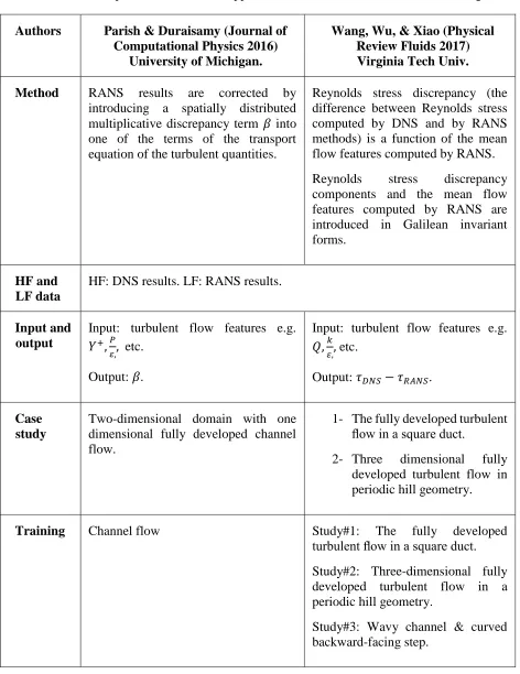
the error in RANS simulation results [26, 27]. A comparison that summarizes these efforts is

presented in Table 1. Both groups made use of High-Fidelity (HF) simulation results from DNS to

correct the Low-Fidelity (LF) model results from RANS. In [26], RANS results are corrected by

spatially distributed multiplicative discrepancy term, 𝛽, into one of the terms of the transport

equation of turbulent quantities; in [27], the Reynolds stress discrepancy is directly based on mean

flow features computed by RANS.

The statistical model in both cases is trained based on the available high-fidelity data and

then tested on other cases, which have a different Reynolds number or a different flow geometry.

Recently, the Virginia Tech University research group suggested that [28] the group of input

features could be increased to more than 50 flow features to improve the prediction capability of

the statistical model. It was also shown that not only could Reynolds stress discrepancy, computed

by RANS, be improved by predicting Reynolds stress discrepancy, but also the improved Reynolds

stress results in a more accurate velocity field. Similarly, Barone et al. [29] used deep neural

(28)

9 Table 1. A Comparison between two approaches for data-driven turbulence modeling.

Authors Parish & Duraisamy (Journal of Computational Physics 2016)

University of Michigan.

Wang, Wu, & Xiao (Physical Review Fluids 2017) Virginia Tech Univ. Method RANS results are corrected by

introducing a spatially distributed multiplicative discrepancy term 𝛽 into one of the terms of the transport equation of the turbulent quantities.

Reynolds stress discrepancy (the difference between Reynolds stress computed by DNS and by RANS methods) is a function of the mean flow features computed by RANS.

Reynolds stress discrepancy components and the mean flow features computed by RANS are introduced in Galilean invariant forms.

HF and LF data

HF: DNS results. LF: RANS results.

Input and output

Input: turbulent flow features e.g.

𝑌+,𝑃

𝜀,, etc. Output: 𝛽.

Input: turbulent flow features e.g.

𝑄,𝑘

𝜀,, etc.

Output: 𝜏𝐷𝑁𝑆− 𝜏𝑅𝐴𝑁𝑆.

Case study

Two-dimensional domain with one dimensional fully developed channel flow.

1- The fully developed turbulent ﬂow in a square duct.

2- Three dimensional fully developed turbulent flow in periodic hill geometry.

Training Channel flow Study#1: The fully developed

turbulent ﬂow in a square duct.

Study#2: Three-dimensional fully developed turbulent flow in a periodic hill geometry.

(29)

10 Table 2 (continued). A Comparison between two approaches for data-driven turbulence

modeling.

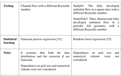
Statistical data-driven models are usually trained on a set of data and then tested with

another group of data that are “close” to the training data in some sense. The “closeness” between

the training data and the testing data can be used to assess the prediction confidence a priori [33].

This closeness could be quantified by metrics like the Mahalanobis Distance [34] or the Kernel

Density Estimation technique [35]. This approach was successful in most cases except when the

training and testing cases are too close or too far apart [33].

ML model predictions, for RANS Reynolds stress anisotropy, for flows of similar physics,

should be similar. ML model predictions should not change with changing the orientation of

coordinate frame. In other words, ML predictions should be Galilean invariant. Based on this

principle, a multi-layer (deep) ANN (also called “deep learning”), with invariant tensor basis, was

proposed [36]. This way, Reynolds stress anisotropy tensor can be predicted with an embedded Testing Channel flow with a different Reynolds

number.

Study#1: The fully developed turbulent ﬂow in a square duct with a different Reynolds number.

Study#2&3: Three dimensional fully developed turbulent flow in a periodic hill geometry with a different Reynolds number.

Statistical learning

Gaussian process regression [31]. Random forest regression [32].

Notes It assumes that both the data distribution and the corrector 𝛽 are Gaussian.

Dependence on grid size and numerical scheme were not considered.

(30)

11 Galilean invariance. The proposed tensor-basis ANN proved to have more accurate prediction

compared to both RANS models and conventional ANN.

1.5.4. Smoothed Particle Hydrodynamics

Data-driven models, for fluid simulations, are used not only in mesh-based CFD but also

in Smoothed Particle Hydrodynamics (SPH) (where Navier-Stokes equations are approximated on

fluid particles instead of a computational grid [21]). Random Forest Regression (RFR) [32] was

trained to predict the velocity and position of the fluid particle in the next time step based on the

velocity and the position in the previous time step [37]. This approach aims to “learn” the behavior

of fluid from the training examples and provides an alternative for real-time fluid simulations.

1.6.CG-CFD for Simulating CTH

Typical accident scenarios may include long transients, CTH multi-physics phenomena,

and the flow regime may change over the computational domain or over time. CG-CFD approach

can be used to deal with such a complex situation, as presented in Figure 1. In Figure 1, a

conceptual framework is proposed to benefit from the fine-grid simulation results, to correct the

CG-CFD results for every single phenomenon, while the multiple-phenomena scenario is

simulated with coarse grids.

In Figure 1, the boxes are numbered from 1 to 8 to refer to 8 steps. In the 1st step, the flow

of every single phenomenon of interest is simulated with a grid which is coarse relative to the grid

requirement of DNS. This coarse-grid simulation is not expected to obtain accurate results, but it

is still expected to show a flow pattern similar to the high-fidelity simulation result. For instance,

in Figure 2, the difference between the coarse-grid and the fine-grid results is clear, both results

show similar flow pattern. Repeating this step with a variety of potential phenomena will result in

(31)

12 Figure 1. A conceptual framework for simulating CTH with CG-CFD. The focus of this work is

highlighted in yellow.

. Since the number of nodes in a fine gird is much larger than in a coarse grid, it is hard to

compare the fine and coarse grid results directly. Instead, coarse-grid results (1st step) are compared

to the fine-grid results (3rd step) mapped on the coarse grid (4th step). Figure 2 gives an example

(32)

13 profile is not perfectly similar to the fine-grid results (especially near the corners of the cavity),

the mapped profile is much more accurate than the coarse-grid one. In this work, machine learning

algorithms are utilized to get a statistical data-driven model that models a correction term (7th step)

that compensates for the information lost due to the coarseness of the grid.

Figure 2. A snapshot of the velocity (𝑈_𝑦) profile in a three-dimensional quasi-steady state turbulent flow in a lid-driven cavity. The lid is moving in 𝑥-direction. The profile is computed with a fine grid (left) and a coarse-grid (right). The fine-grid result is mapped to a coarse-grid (in the middle).

Based upon the success of the first 4 steps, simulating a realistic nuclear accident scenario

that involves multi-phenomena with a coarse grid can be beneficial (5th step). Given the

non-accurate predictions coming out of the 5th step plus the library created in the 2nd step, different

phenomena involved in a containment scenario can be identified (6th step: pattern recognition).

Pattern recognition is a process of classifying the features into groups. It may help to distinguish

(33)

14 If each phenomenon is identified correctly, it may be possible to benefit from the correction

term computed in the 7th step to correct different group of results corresponding to different

phenomena. It would be challenging to use correction terms computed by different data-driven

models for different groups of interacting phenomena. Therefore, blending functions may be

needed to deal with a mixture of models (8th step).

1.7.The Scope of This Work

Since the traditional high-resolution (mesh-independent) CFD solution is computationally

expensive and using of a coarse grid would result in high grid-induced errors, the present work

focuses on predicting the errors of the coarse-grid solution. While the previous research aimed

largely to reduce the model form error, in this work, the sub-grid effect is compensated for by a

surrogate statistical model that is trained by using high-fidelity simulation results (fine-grid CFD).

The objective of this work is to investigate the feasibility of obtaining a correction for the

CG-CFD simulation results using machine learning algorithms. Numerical experiments are

designed and performed to study the feasibility of utilizing machine learning tools to get a

correlation between the ‘correct’ solution informed by fine grid simulation results and the

coarse-grid variables. Among the different sources of error in CFD simulation (see Figure 3), the

turbulence modeling error and the discretization error are the most challenging ones. Below, in

Subsections 1.7.1, 1.7.2 and 1.7.3, the present work is compared to other CFD approaches in terms

(34)

15 Figure 3. CFD sources of error.

1.7.1. Present Approach vs. Traditional CFD

RANS turbulence models are popular because of the reduced computational expense while

representing three-dimensional flow behavior. RANS turbulence models typically rely on

incorporating more physics and using empirical models for some parameters based on the available

(35)

16 study), but this grid convergence study should be applied within the range of grids that satisfy the

turbulence model grid requirements. Typically, for each new case, a new simulation is needed,

even if the new case is only slightly different from old cases.

In the present work, the “No model” approach (where NS equations are solved numerically

without any turbulence model) is utilized with coarse grids (discretization grids that are expected

to produce non-accurate results). However, instead of investigating the turbulence modeling error,

we use the same “No model” approach with different grids (fine and coarse grids) to train a

surrogate model to compute this grid-induced error. The CG-CFD error is predicted by comparing

the high-fidelity results (with fine grids) against CG-CFD results. With this surrogate model, the

grid-induced error can be predicted for other cases that have different grid sizes, Reynolds

numbers, etc. The surrogate model is adaptive with the available data, so each new set of

experimental data or high-fidelity computations will be reflected in the automatically-improved

model, without the need for developing other models that capture the new data.

1.7.2. Present Research vs. Turbulence Modeling Error Reduction

Recently, research has been pursued in the direction of taking advantage of the ML

algorithms to develop surrogate models that can compute the turbulence modeling error (for

instance, [26, 27]). This approach is known as Physics Informed Machine Learning (PIML)

approach. Both the present work and PIML method benefit from ML algorithms to produce

data-driven statistical models. PIML recent research assumes that one of the RANS models is used and

the grid convergence criterion for this model is satisfied. Through PIML, the difference between

RANS flow variables profile and DNS profile is computed. On the other side, the present work

depends on the same NS equations used with both fine and coarse grids. After that, the error

(36)

17 1.7.3. This Work vs. Reduced Order Modeling (ROM)

ROM techniques can be categorized in two classes: dimensionality reduction and surrogate

modeling [38]. The first class is the dimensionality reduction techniques which aim to reduce the

number of inputs or (dimensions) of the model without changing the original function. CG-CFD

approach discussed in this work does not involve any dimensionality reduction because the same

flow variables are included in both fine and coarse-grid simulations.

The second class is the surrogate modeling which leads to substituting the original model

with another approximate more simplified function. This simplification is either based on physics

or based on statistics (data). For instance, LES and RANS method can be regarded as

physics-based approaches because both methods were developed physics-based on some physical assumptions and

are considered as approximations of the original NS equation. On the other side, the

statistics-based surrogate functions are selected heuristically by regression methods or ML algorithms. To

classify the current work, the proposed CG-CFD approach is described symbolically as follows:

The discretized NS equations solved on a sufficiently fine grid is written as: 𝐿_𝑓(𝜑) = 0.

𝜑𝑓 is the flow variables computed by the fine grid and 𝐿𝑓 is the discrete operator computed by a fine grid. The discretized CG-CFD equations can be written as 𝐿_𝛥(𝜑_𝛥) = 0. 𝛥 is the cell length of the coarse grid. The grid-induced error, when computing a variable 𝜑, is 𝜀_𝛥(𝜑) = 𝜑_𝑓→𝛥− 𝜑_𝛥, while 𝜑𝑓→𝛥 is the 𝜑𝑓 field mapped on a coarse grid. Using ML, a surrogate function 𝐹 is computed:

𝜀_𝛥(𝜑) = 𝐹(𝑋(𝜑_𝛥)) (1-1)

where X(𝜑_𝛥) is the features set (new variables) computed given 𝜑_𝛥. The process of obtaining

(37)

18 1.8.The Structure of This Dissertation

Sources of uncertainty in CFD are mainly turbulence modeling error and numerical error

(see Chapters 2 and 3, respectively). The numerical error (in particular, the grid-induced error) is

recovered using data-driven techniques based on ML. Different ML algorithms are listed in

Chapter 4. These ML algorithms are utilized to produce a statistical model that can predict the

CFD coarse-grid-induced error, given the flow features computed by a coarse grid (see Chapter

5). The capability of the statistical model to predict the grid-induced error in different cases is

illustrated and assessed in Chapter 6. The conclusion of this dissertation and the future work plan

are provided in Chapter 7. The following section (Section 1.9) is presented to clarify the meaning

of some terms used in the context of this work.

1.9. Definitions

• Training data: A set of data needed to discover the relationship between different variables.

For instance, this group of data is used to find the regression function which relates the output

and input.

• Testing data: After training the statistical model given the “training data”, this model is

assessed using the testing data. Testing data are totally independent of the training data.

• Features: (or attributes or inputs) are the input variables which characterize the problem. For

instance, fluid flow features can be the velocity or the pressure and so on.

• Discretization error: the difference between the exact solution of the discretized equation and

the exact solution of the original Partial Differential Equations (PDEs). It includes both

truncation error (locally generated) and the pollution error (transported component).

• Truncation error: when approximating a function by a summation (for instance, Taylor series),

(38)

19 and it occurs when truncating the infinite series used to approximate a PDE (when discretizing

PDEs). This error is eliminated by refining the grid. Truncation error is the local source of the

discretization error.

• Pollution error: It is another component of the discretization error. It is not produced locally

but transports from elsewhere in the computational domain. This error is transported through

the domain similar to the solution transport (the error can be convected or diffused).

• Round-off error: Difference between the actual number and its approximation (rounding)

stored on the computer. This error is assumed to be small compared to other errors.

• Iterative convergence error: it is an error that results from the iterative algorithm that is used

during the simulation. Typically, this iteration is stopped based on a criterion (typically the

residual). It is the difference between the solution of the discretized equation with the stopping

criterion and the exact solution of the discretized equation with a zero residual.

1.10. Chapter Summary

Modeling and simulation of Containment Thermal Hydraulics (CTH) phenomena are

achieved either by system codes or Computational Fluid Dynamics (CFD). Affordable

computations on the reactor-system level are performed by system codes using large control

volumes (larger than one cubic meter). Using System codes, CTH phenomena are modeled

with different degrees of dimensionality. Although system codes represent the currently

available knowledge in the nuclear industry, they cannot properly model the complex

multi-dimensional behavior of CTH phenomena because of the uncertainty related to the used

empirical equations, empirical parameters, simplified geometries and coarse-mesh resolution.

On the other side, CFD codes can model phenomena which are multi-dimensional, local,

(39)

20 applying CFD would be a huge computational challenge when modeling complex accidents

with long transient scenarios.

This work is motivated by the need to mitigate CFD computational expense and the

current progress in data-driven modeling using machine learning algorithms that can benefit

from the available high-fidelity simulations and experimental data. Hence, it is proposed to

rely on the coarse-grid CFD simulations (which are affordable) while the grid-induced error

can be predicted using data-driven models.

Currently, data-driven models (trained by Direct Numerical Simulations (DNS) data)

are utilized in the context of CFD to correct Large Eddy Simulations (LES), Reynolds

Averaged Navier-Stokes (RANS) simulations or to compute closure terms for averaged

variables’ equations. On the other side, the present work investigates the feasibility of

correcting coarse-grid solutions computed by Navier-Stokes equations, without turbulence

modeling, using data-driven models that are trained with sufficiently fine-grid simulations.

A method that predicts the grid-induced error given the coarse-grid solution features is

proposed. Currently, this method is applied to a turbulent three-dimensional flow inside a

cavity. A General framework that benefits from the proposed method to simulate CTH

phenomena using coarse-grid CFD is also proposed in this work.

(40)

21

2. TURBULENCE MODELING

CFD approach is used in CTH analyses to capture the relevant multi-dimensional

phenomena in detail. CFD implies solving Navier-Stokes equations numerically and this requires

finer grid resolution especially if the flow is highly turbulent. CTH phenomena typically include

turbulent flows, therefore, solving NS equation directly will be computationally expensive due to

fine-resolution requirements. After clarifying the objectives of this chapter (Section 2.1), basic

turbulence theory is introduced briefly (Section 2.2). The methods which are typically used to

model turbulence are presented (namely, LES (Section 2.3) and RANS (Section 2.4)). This chapter

gives the reader an overview of the traditional mechanistic turbulence model used to mitigate the

need for high-resolution grids. The confidence in either LES or RANS simulations is related to

reducing CFD sources of error (See Figure 3). Among these sources of error, grid induced-error is

the focus of this work as we propose to rely on coarse-grid simulations. Hence, the grid-induced

error, in the simulations performed by LES, RANS and the proposed CG-CFD method, is

discussed in Section 2.5 and the whole chapter is summarized in Section 2.6.

2.1.Objectives

The objectives of this chapter can be summarized as follows:

• Discussing the traditional mechanistic turbulence models.

• Providing an overview of the grid-induced error treatment in the proposed CG-CFD

method vs. the corresponding error when applying traditional turbulence modeling.

2.2.Basics of the Turbulence Theory

Turbulence is unsteady and chaotic fluid motion in which the three velocity components

fluctuate mixing matter, momentum, and energy. Turbulent flows always occur at higher Reynolds

(41)

22 eddies of different sizes. There are large scales where the energy enters the flow through mean

shear; there is an inertial range (intermediate scales) where energy flows to the smaller scales of

the dissipation range where the energy dissipates into heat due to molecular viscosity effects [12].

A typical example of the distribution of turbulence energy contained in the eddies of size 𝑙

(corresponding to wavenumber 𝜅𝑙 = 2𝜋

𝑙) is illustrated in Figure 4.

Figure 4. Distribution of turbulent energy in wavenumber space.

In order to represent the eddies belonging to various energy ranges, NS equations can be

solved directly on a sufficiently fine grid using a small-time step to capture length scales down to

Kolmogorov length scale (𝜂) and time scales down to 𝜏η:

𝜂 = (𝜈3_{⁄ )}e 1 4⁄ _(2-1)

(42)

23 This method (Direct Numerical Simulation, DNS) is the most accurate method of solving

turbulent flows. It results in accurate three-dimensional instantaneous velocity and pressure

numerical data. It is accurate for simple flows, but it is computationally challenging for real-world

applications (turbulent flows with higher Reynolds number, Re). The number of grid points needed

for DNS simulation is proportional to Re9/4 [12] (see Figure 5). For most applications, it is unnecessary to resolve all the turbulence scales. It suffices to predict the effect of turbulence on

mean flow behavior. Therefore, turbulence models are developed to close the system of the mean

flow equations. Different turbulence modeling methods are described in Sections 2.3 and 2.4. It is

worth noting that the averaged flow pattern is a statistical flow property (cannot be directly

observed in nature for turbulent flows).

2.3.Large Eddy Simulation (LES)

LES method was proposed by Smagorinsky [16]. In this method, turbulent flow large

eddies are resolved directly while the sub-grid scale eddies (the ones which cannot be resolved

using the coarser grid) are modeled. This results in the reduced computational cost of LES

compared to DNS. LES requires the smallest resolved spatial and temporal scales to lie in the

inertial subrange of turbulence (see Figure 4). Large eddies contain most of the turbulent kinetic

energy and are responsible for turbulent mixing and momentum transfer while the small eddies are

isotropic (universal and less dependent on boundary conditions) which allows developing a nearly

universal sub-grid model for them. The computational cost of LES (for free shear flow simulations)

varies weakly with Reynolds number and is proportional to 𝑅𝑒0.4 [39]. For wall-bounded flows, LES computational cost (number of grid points) scales with 𝑅𝑒1.76_{[39] (this computational cost} is comparable to DNS as illustrated in Figure 5) . Thus, LES method allows to perform simulations

(43)

24 In LES, any variable in NS equation, 𝜑 is spatially filtered to resolve the large turbulent

eddies whose scales range from domain size to filter width while the eddies of scales between filter

size and grid width are modeled. The filters are localized functions that include Gaussian filtering,

box filtering (simple average over volume) and cutoff filtering (Fourier coefficients belonging to

wavenumbers above the cutoff are eliminated). For example, using a box filter, the filtered variable

𝜑̅ is given by:

𝜑̅(𝑥) = 1

𝑉∫𝑣𝜑(𝑥′)𝑑𝑥′, 𝑥′ ∈ 𝑣 (2-3)

where 𝑉 is the volume of a computational cell. The filtered NS equation (for incompressible flow)

is: 𝜕𝑢̅𝑖 𝜕𝑡 + 𝜕𝑢̅ 𝑢_𝑖̅_𝑗 𝜕𝑥𝑗 = 𝜕 𝜕𝑥𝑗 (𝜕𝜎̅̅̅̅𝑖𝑗 𝜕𝑥𝑗 ) −𝜕𝑝̅̅̅𝑘 𝜕𝑥𝑖 −𝜕𝜏̅̅̅𝑖𝑗 𝜕𝑥𝑗 (2-4) 𝜎_𝑖𝑗 ̅̅̅̅ = 𝜈 (𝜕𝑢̅𝑖 𝜕𝑥_𝑗+ 𝜕𝑢̅_𝑗 𝜕𝑥_𝑖) − 2 3𝜈 𝜕𝑢̅_𝑖

𝜕𝑥_𝑙𝛿𝑖𝑗 (2-5)

𝜏_𝑖𝑗

̅̅̅ = 𝑢̅̅̅̅̅ − 𝑢_𝑖𝑢_𝑗 ̅ 𝑢_𝑖̅_𝑗 (2-6)

where 𝑝_𝑘 and 𝜈 are the kinematic pressure and kinematic viscosity. 𝜏̅̅̅_𝑖𝑗 is the Sub-Grid Scale (SGS) stress tensor. One of the earliest models to solve 𝜏̅̅̅𝑖𝑗 is the Smagorinsky turbulence model [16]. Similar to the dissipation due to dynamic fluid viscosity in a laminar flow, the concept of SGS

viscosity, 𝜈𝑠𝑔𝑠, is introduced to represent the dissipation effect of small scales as following:

𝜏_𝑖𝑗 ̅̅̅ −1

(44)

25

𝑆𝑖𝑗

̅̅̅̅ = 0.5 (𝜕𝑢̅𝑖

𝜕𝑥𝑗

+𝜕𝑢̅𝑗 𝜕𝑥𝑖

) (2-8)

𝜈_𝑠𝑔𝑠 = 𝐿2_𝑠𝐶_𝑠2|𝑆| (2-9)

𝑆 = √2𝑆̅̅̅̅𝑆_𝑖𝑗̅̅̅̅_𝑖𝑗 (2-10)

𝐿_𝑠 = 𝑚𝑖𝑛 [𝜅𝑦

𝐶_∆(1 − 𝑒

−𝑦+

𝐴+_{) , 𝑉}1/3_] _(2-11)

where 𝑆̅̅̅̅_𝑖𝑗 is the strain rate of the resolved velocity field, 𝐿_𝑠 is the mixing length for sub-grid scales and 𝐶𝑠 is a model constant (proposed to be 0.18) [40]. The SGS viscosity value is large near the wall because of the high velocity gradient at the wall. Near wall turbulent fluctuations go to zero

so 𝜈𝑠𝑔𝑠 must go to zero as well. Therefore, Van Driest damping [41] is added (Eq. (2-11)). In this equation, 𝜅 is the von Karman constant, 𝑦 is the closest distance to the wall, 𝐶∆ and 𝐴+ are model constants, 𝑉 is the computational cell volume. This model has some limitations because 𝐶_𝑠 value needs to be changed for different flow patterns. It may take values from 0.065 to 0.25 [42].

To eliminate the need for tuning Smagorinsky constant, a dynamic model is developed by

Germano and Lilly to [40] compute the Smagorinsky constant dynamically. In this model, the flow

variables are filtered by 2 filters (grid filter and test filter) while the test filter is larger than the grid

filter width. Filtering with a grid filter results in SGS tensor, 𝜏̅̅̅𝑖𝑗 (see Equation (2-6)). Computing the SGS tensor based upon test filter gives 𝜏_𝑖𝑗𝑡_{. Applying both filters (grid filter and test filter)} yields another SGS tensor, 𝑇_𝑖𝑗:

(45)

26

𝐿_𝑖𝑗 = 𝑇_𝑖𝑗 − 𝜏_𝑖𝑗𝑡 (2-13)

𝑀_𝑖𝑗 = −2∆2_(𝛼2_𝑆 𝑖𝑗

̿̿̿̿ |𝑆|̿̿̿̿ − 𝑆̅̅̅̅|𝑆|̅̅̅̅̅̅̅)𝑖𝑗̅̅̅̅ (2-14)

𝐶_𝑠2 = 〈𝐿𝑖𝑗 𝑀𝑖𝑗〉

〈𝑀_𝑖𝑗𝑀_𝑖𝑗〉 (2-15)

where ∆ the test is scale and 𝛼∆ is the resulted scale from applying the two filters. This model

assumes that Smagorinsky constant value at ∆ and 𝛼∆ is the same (scale invariance). In this way,

𝐶𝑠 can be computed for each grid cell and each time step. However, this may cause 𝜈𝑠𝑔𝑠 value to be negative in some locations [43]. In general, LES is capable of simulating separated flow but it

is not affordable when simulating near-wall flow at high Reynolds numbers. The filtered variables

are not averaged over time, so the flow variables are functions of time. Therefore, LES can

compute transient flows. LES is still much more expensive than RANS which is the most used

approach in industrial CFD (see Section 2.4). As depicted in Figure 5, the number of grid points

(46)

27

Figure 5. Computational expense (of DNS, LES, and RANS) as a function of Reynolds number.

2.4.Reynolds Averaged Navier-Stokes (RANS) Equations

RANS is the workhorse tool in turbulence modeling in industry. Reynolds decomposition

of the velocity into a mean velocity component and a turbulent fluctuating component is written

as:

𝑢 = 𝑢 + 𝑢′ _(2-16)

The same way of decomposition is applied to pressure. Applying Reynolds decomposition on NS

Equation (2-17) results in RANS Equation (2-18).

1.E+00 1.E+02 1.E+04 1.E+06 1.E+08 1.E+10 1.E+12 1.E+14

1.E+04 1.E+05 1.E+06 1.E+07

(47)

28 𝜕𝑢_𝑖 𝜕𝑡 = −𝑢𝑗 𝜕𝑢_𝑖 𝜕𝑥𝑗 −1 𝜌 𝜕𝑝_𝑘 𝜕𝑥𝑖 + 𝜈 𝜕 2_𝑢 𝑖 𝜕𝑥𝑗𝜕𝑥𝑗 (2-17) 𝜕𝑢_𝑖 𝜕𝑡 = −𝑢𝑗 𝜕𝑢_𝑖 𝜕𝑥_𝑗− 1 𝜌 𝜕𝑝̅̅̅_𝑘 𝜕𝑥_𝑖 + 𝜈

𝜕2_𝑢 𝑖

𝜕𝑥_𝑗𝜕𝑥_𝑗−

𝜕𝑢𝑖′𝑢𝑗′

̅̅̅̅̅̅̅̅̅

𝜕𝑥_𝑗 (2-18)

NS Equation (2-17) is expressed in tensor notation (for incompressible Newtonian fluid). The right

side of the equation is the momentum time rate of change while the right-hand side is the

summation of the inertial force term (momentum transport because of the bulk fluid motion), the

pressure force and the viscous force. In RANS Equation (2-18), the last term of the right-hand side

is called Reynolds stresses [12]. This term is modeled according to Boussinesq approximation that

Reynolds stresses are proportional to the velocity gradient of the mean flow:

𝑢_𝑖′_𝑢 𝑗′ ̅̅̅̅̅̅ = 𝜈_𝑡(𝜕𝑢𝑖 𝜕𝑥_𝑗+ 𝜕 𝑢_𝑗 𝜕𝑥_𝑖) − 2

3𝑘𝛿𝑖𝑗 (2-19)

𝛿𝑖𝑗 = {

1, 𝑖 = 𝑗

0, 𝑖 ≠ 𝑗 (2-20)

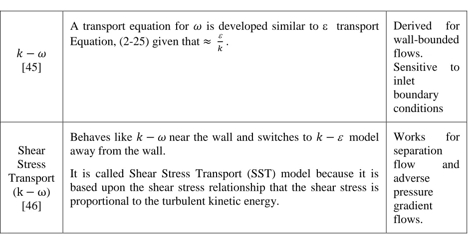
where 𝑘 is the turbulent kinetic energy and 𝜈_𝑡 is the turbulent viscosity. The closure problem is to model 𝜈𝑡. An overview of the common RANS turbulence models that predict 𝜈𝑡 are listed in Table 3. All these models (LES or RANS) still lack accuracy or/and affordability when simulating

complex long transient flows similar to CTH flows. These models are also calibrated on limited

data. Hence, data-driven statistical models developed by ML algorithms (see Chapter 4) are