Real-time video processing using contour numbers and angles for non-urban road marker classification

ISSN: 2088-8708, DOI: 10.11591/ijece.v8i4.pp2540-2548  2540

Real-Time Video Processing using Contour Numbers and

Angles for Non-urban Road Marker Classification

Zamani Md Sani1, Hadhrami Abd Ghani2, Rosli Besar3, Azizul Azizan4, Hafiza Abas5

1

Faculty of Electrical Engineering, Universiti Teknikal Malaysia Melaka, Malaysia

2,3

Faculty of Engineering and Technology, Multimedia University, Malaysia

4,5

Advanced Informatics School, Universiti Teknologi Malaysia, Malaysia

Article Info ABSTRACT

Article history:

Received May 9, 2018 Revised Jun 20, 2018 Accepted Jul 11, 2018

Road users make vital decisions to safely maneuver their vehicles based on the road markers, which need to be correctly classified. The road markers classification is significantly important especially for the autonomous car technology. The current problems of extensive processing time and relatively lower average accuracy when classifying up to five types of road markers are addressed in this paper. Two novel real time video processing methods are proposed by extracting two formulated features namely the contour number, , and angle, 𝜃 to classify the road markers. Initially, the camera position is calibrated to obtain the best Field of View (FOV) for identifying a customized Region of Interest (ROI). An adaptive smoothing algorithm is performed on the ROI before the contours of the road markers and the corresponding two features are determined. It is observed that the achievable accuracy of the proposed methods at several non-urban road scenarios is approximately 96% and the processing time per frame is significantly reduced when the video resolution increases as compared to that of the existing approach.

Keyword:

Auto assist driving system Road marker classifications Video image processing

Copyright © 2018 Institute of Advanced Engineering and Science. All rights reserved.

Corresponding Author:

Zamani Md Sani,

Faculty of Electric and Electronic, Universiti Teknikal Malaysia Melaka,

Hang Tuah Jaya, Durian Tunggal, 75450, Malaysia. Email: [email protected]

1. INTRODUCTION

The number of road accidents in Malaysia increases at an alarming rate of 9.7% every year over the past thirty years [1] contributed by (road users) errors, faulty road environment, and vehicle defects. The road marker, is very important in guiding road users while driving. Different types of road markers in non-urban roads such as double solid (DD), dashed (D), solid-dashed (SD), dashed-solid and single solid (SS), allow drivers to safely decide either to maintain the course in the middle of the lane or to overtake the front vehicles. In earlier works, many efforts were invested in solving lane detection and tracking problems for Auto-Assist Driving System (ADS) [2], [3]. These methods had been used as a warning system to the driver [4]-[8] and surprisingly, the lane detection also was used as part of the system to analyse the driver behaviour [9]. Symbols, alphabets, and custom markers were also being explored and used as the information to alert drivers [10,11].

spectrum and Fourier analysis to detect three types of markers, which are; single solid, dashed, and merged road markers. However, road marker classification for non-urban type roads was not addressed. Schubert et al. [15] studied lane changing based on road marker recognition surrounding traffic situation but the road markers classified were limited to only; dashed and solid lines. In a work by Lindner et al. [16], an edge detector technique was designed to subsequently search for a group of four objects namely the lines, curves, parallel curves and closed objects in detecting road markers. Although four types of road markers were classified, most of the road markers are dashed lines with different sizes.

Meanwhile, another research from Suchitra et al. classified three road markers namely; dashed, solid and zigzag using a modular approach [17]. The road markers are classified as either dashed or solid using the Basic Lane Marking (BLM), which is based on continuity properties. This approach however, applies the temporal information in the classification operation, which renders slower detection when the road marker type changes whilst driving on the road. In addition to these methods, Nedevschi et al. [18] uses a periodic histogram to determine the type of road markers. This ego-localization is observed to enable the classification of road markers into four types namely single solid, double solid, dashed, and merged.

In a recent research, Paula et al. [19] presented an automatic classification technique to classify five types of road markers. The approach uses between three to five features extracted from the image, which is later fed to the artificial neural network. A two-stage method is modelled for the full classification, with the first stage applies the Bayesian classifier for dashed, single dashed and double solid while the second stage differentiates between dashed-solid and solid-dashed lines for road marker detection. However, the results of the classification were found to have changed abruptly on each frame, which caused inconsistent results while driving. Mathibela et al. [20] proposed a new approach using a unique set of geometric features which functions within a probabilistic RUSBoost and Conditional Random Field (CRF) network to classify the road markers into seven types, including; single boundary, double boundary, separator, zig-zag, intersection, boxed junction and special lanes. Even though more types of road markers were classified using this method, unfortunately, the classification only used static images in urban roads.

On the basis of the comprehensive literature review, the extensive classification of road markers had been rarely studied. It is interesting to look at the aforementioned different approaches for road marker classification although no standard databases available to allow fair comparison. In addition, the dimension, colour and size of the markers are varied across the world.

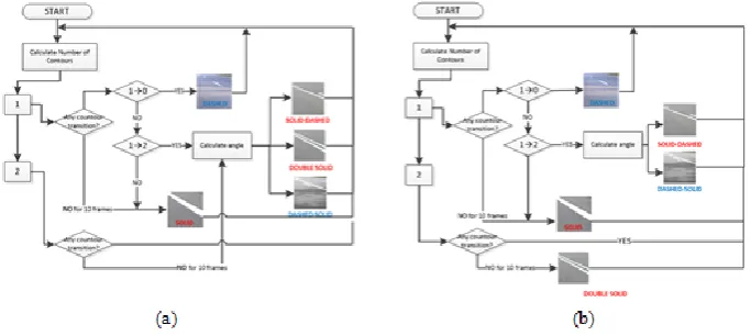
This paper proposes a novel approach to classify these road using a customized Region of Interest (ROI) in a video acquired from a camera with its calibrated position. Two features are derived, namely; the contour number, , and the contour angle, 𝜃, are later fed into a two-layer classifier. The first layer classifies the D and SS marker types based calculated , values, while the second layer classifies the DD, DS or SD marker types, by using 𝜃 values as shown in Figure 1. Temporal information integration is applied to improve the classification accuracy by validating the marker type’s transitions on the road. This algorithm has been demonstrated an overall accuracy of approximately 95% and reduced reduction in the processing time by ~50% shorter than the existing method.

Figure 1. Road markers found at two-way non-urban road

2. RESEARCH METHOD

2.1. Camera setup for region of interest selection

Many existing methods for selecting the ROI such as the vanishing point, area-based detection and area-based tracking methods had been used in the past. A technique of calculating the vanishing point using Hough Transform (HT) is carried out by obtaining the intersection line and the ROI at the lower half of the image [21]. In [22], [23], the ROI is selected over the whole horizontal axis and a limited range along the vertical axis, before the feature extraction and road marker or lane classification take place.

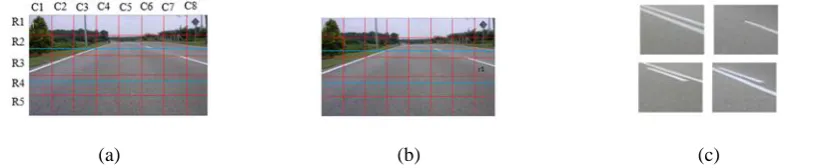
horizontal lines, h1 and h2, are set on the FOV to equally divide into three sections as in Figure 2(c), where the h1 horizontal line in the image must be at the same level with the most right lane in the image.

(a) (b) (c)

Figure 2. The camera setup (a) Camera position (b) 3d camera coordinate system (c) Camera height adjustment with h1 and h2 horizontal lines

The image captured is then divided into 40 equally sized sections or squares, each of which having a size of 160x144 pixels as shown in Figure 3(a) and Figure 3(b). The ROI selection method is applied to every video frame to choose (x,y) as the ROI, which contains the road marker, as shown in Figure 3(c). It can be observed that (x,y) is the nearest to the car where the effects of the road curve on the road marker is low. In the case of lane departure, the ROI will contain no marker for a longer duration which indicates that the vehicle is departed from the right track. In our approach, r1, containing the RGB information, is converted to

greyscale and filtered through Gaussian filter [24] before undergoing the thresholding process using Otsu Thresholding method [25] for binary conversion. Then the two features, which are the contour number and the angles, will be extracted to complete the classification as discussed next.

(a) (b) (c)

Figure 3. (a) Row and column post camera position calibration (b) ROI r1 (c) ROIs consist of road markers

2.2. The number of contours, , and the angle 𝜃 in Method A and B

A contour is a line that connects all points along the boundary of an object of the same colour. The contour number, in the ROI is calculated by counting the number of all contours along its horizontal axis. The calculation of is carried out in the ROIs, (x,y), for every frames in a complete cycle, which is defined as the time taken by all consecutive frames containing a complete road marker pattern. This pattern will repeat itself after every complete cycle until the road marker type changes or ends as in Figure 4. The proposed road marker classification is based on the contour number, , and the contour angle, 𝜃, implemented using two methods of two-layer classification as depicted in Figure 5. The formulation

of and 𝜃 for both of these methods, which are named as Method A and Method B, will be presented

next.

In Method A, road marker D is detected when the minimum over the cycle is zero and the maximum is one. If over a complete cycle, then the road marker is SS. Otherwise, if the maximum over the cycle is two, then the second layer classification using the angle 𝜃 of the centroids will be run to classify the marker as SD, DS or DD. The angle θ, which is measured between a line connecting the two centroids and the horizontal axis, is calculated only on the first frame in a set of frames showing a particular road marker pattern that repeats itself after the last frame in the set before the pattern changes. This can be identified from the change in value, which is from 10 or 12. There arethree threshold angles 𝜃 𝜃 and 𝜃 , which are determined from training dataset, applied for the

(a)

(b)

Figure 2. The contour number calculated from the frames (a) Dashed (b) Solid-dashed

Figure 5. Two-layer classification diagram (a) Method A (b) Method B

In Method B, the significant different is when detecting DD. Instead of detecting DD at the second layer using the angle 𝜃, DD is detected at the first layer based on , when it is equal to two over a complete cycle. Hence, only one threshold angle, 𝜃 , used to detect DS and SD. In order to find the contour

angle, as seen in Figure 6 (d) and formulated as follows:

𝜃 [ ] (1)

Two centroids, and , are calculated from the moments of the markers,

,

,

the contours and the red dots denote the centroids. The moments are calculated as

∑ , where represents the region in the contour (the red lines) [26].In the

next section, the threshold angles 𝜃 will be determined to classify the road marker as DD, DS or SD (for

(a) (b) (c) (d)

Figure 6. (a)-(c) ROI with centroids found (d) 𝜃 value calculation from two centroids

2.3. The threshold angles formulation for the second-layer classification in method A and B In Method A, the threshold angles 𝜃 are formulated based on the angles 𝜃 between two centroids

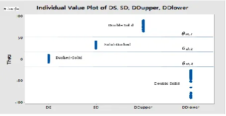
of each of the 300 frames extracted from four video clips (Vid22_USB, Vid24_USB, Vid26_USB, Vid27_USB) as in Table 2. Theangles 𝜃 are then plotted accordingly in Figure 7. As for DD, the 𝜃 values are found to be distributed between the negative angles (denoted as DDlower) and the positive angles (denoted as DDupper) due to the change in the location of the two centroids shifting along a curvy road. The angles 𝜃 for the 1st

frames in every set of frames for DS, SD and DD are found to be separated with each other, as seen in Figure 7. It is clear from this figure that the threshold angles, 𝜃 are the separating angles

or lines between four groups of angles where for Method A.

Figure 3. Distribution of the 𝜃 for 𝜃

The three threshold angles, 𝜃 𝜃 and 𝜃 which are represented by the blue horizontal lines

in Figure 7, are calculated such that the angles or 𝜃 values are separated or classified intro three types; namely DD, SD and DS. Hence, these threshold values the midpoint between the maximum angle of a marker type and the minimum angle of the next neighbouring marker type. The minimum and maximum angles of DDupper, SD, DS and DDlower are stored as the first row (minimum angles) and the the second row (maximum angles) of matrix respectively. Based on the 𝜃 values recorded in Figure 7, the corresponding matrix is given below.

where the threshold angles are calculated using the following formula

𝜃

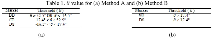
with 𝜃 °, 𝜃 and 𝜃 , as shown in Table 1 (a) for making the classification

Table 1. 𝜃 value for (a) Method A and (b) Method B

(a) (b)

2.4. Resolving errors in classification

Errors in road marker classification tend to happen during the marker transition period. The frame delay time might also cause errors in classification. Both of these cases can be solved by using the temporal information between the classification results during the transition period. The markers tend to be similarly labelled for a set of adjacent frames. Knowing this tendency, the previous set of classification result will be stored and if there is a transition of marker types, it will wait on the next set of frames classification results for a final validation to avoid unnecessary classification errors.

3. RESULTS AND ANALYSIS

The proposed algorithm was tested with multiple video sequences captured by two different devices with different car velocities using a lower range USB camera (Logitech c310) and a higher range camera (GoPro Hero Silver). To evaluate the robustness of the new algorithm, other sets of videos acquired with different devices at different resolutions and the velocity of the vehicle is between 60-90 km/h for the test video images, which meets the speed limit in the suburban road area. The videos are also taken when the vehicle was moving on different road conditions including flat, hilly and narrow roads. The videos used to determine the threshold angles were taken with a moderate vehicle speed between 50-60 km. The experiments were carried out using a desktop computer equipped with Intel® core ™ i7-4790 CPU @360GHz and 16 GB RAM. The proposed system was implemented by using the Visual Studio C++ 2010 compiler with the library from OpenCV version 2.4.11.

In the classification process, if , the software will classify it as either D or SS depending on found in the next set of frames. For example, if the next set of frames detected with , the system will classify it as a D types whereas if consistently detected over the complete cycle, the system will classify it as SS types. If the maximum value is two over the complete cycle, the road marker will be classified as either DS, SD or DD, by using the 𝜃 value calculated at the 1st

frame from the set of frames. The classification result will remain and will only be reclassified if , changes from 21. For the case of DD type which expects consistently, a sampling up to its 10th frames will be performed when only two contours are detected and classification result will be updated by using the 𝜃 value on its 11th frame.

The accuracy of the marker classification is calculated using Equation (3). The total sets of frames classified correctly, Ʃ⍴, will be divided by the total sets of frames in the video image Ʃξ, excluding the total number of 1st sets of frames when the road marker transition happens, Ʃτ1. The exclusion of Ʃτ1 is due to the road marker transition in which the angle 𝜃 calculation is temporarily paused. The clips and the accuracy results are shown in Table 2.

∑ ⍴ ∑ _{∑ ∑} (3)

As shown in Table 1, clips 4 to 7 were trained for identifying 𝜃 . Clips 9 and 10 are recorded

Table 2. Clips Information and the Accuracy Results for both methods

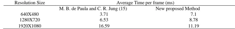
Table 3: Average Time Execution for Each Frame

Resolution Size Average Time per frame (ms)

M. B. de Paula and C. R. Jung (15) New proposed Method

640X480 3.71 7.1

1280X720 6.53 8.78

1920X1080 16.59 11.19

4. CONCLUSION

A novel approach on the road markers classification process is presented in this paper. A smaller ROI is used to process the video frames and extract the formulated features, which are the contour number and angle, as the inputs for the proposed two-layer classifier algorithm. The average accuracy of ~96% has been achieved using our proposed algorithm, with a relatively lower processing time per frame at large video resolution as compared with the existing approach. The errors found in the road marker classification are caused by the abrupt changes in illumination, vanishing road marker, white elements on the road and markers blocking by the other vehicles. Future work will focus on the illumination and faint marker issues that affect the features extraction for classifying the road marker types.

ACKNOWLEDGEMENTS

The authors would like to acknowledge the funding support received from Universiti Teknikal Malaysia Melaka (UTeM) from PJP/2014/FKE(15D)/S01357 – Road Lane Recognition Using Vision and Artificial Intelligence for Auto Assist Driver Alert System. In addition, a special thanks to Universiti Teknologi Malaysia (UTM) for funding this paper under PAS Grant Number PY/2016/07732. The authors also would like to acknowledge Mohammed Fauzi Mohammed Hussein as an industry expert who has given advice and support throughout the full project completion.

REFERENCES

[1] Mustafa, M. N., “Overview of Current Road Safety Situation In Malaysia”, Highway Planning Unit, Road Safety Section, Ministry of Works, 2005.

[2] Mita, S., & McAllester, D., “Lane detection and tracking in challenging environments based on a weighted graph and integrated cues”, 2010 IEEE/RSJ International Conference on Intelligent Robots and Systems, pp. 5543-5550, 2010.

[3] Zhe, X., & Zhifeng, L., “A robust lane detection method in the different scenarios”, 2012 IEEE International Conference on Mechatronics and Automation, pp. 1358-1363, 2012.

[4] Fan Chao, Xu Jing-bo & DI Shuai, “Lane Detection Based on Machine Learning Algorithm”, TELKOMNIKA (Telecomuunication, Computing, Electronics and Control), vol. 12-2, pp. 1403-1409, 2014.

[5] Chunyang Mu, Xing Ma., “Lane Detection Based on Object Segmentation and Piecewise Fitting”,

TELKOMNIKA

[6] Xiaodan Huang, Wei Wang., “Traffic Prediction Based on Correlation of Road Sections”, TELKOMNIKA (Telecomuunication, Computing, Electronics and Control), vol. 11, no. 10, pp. 5523-5529, October 2013.

[7] Son, J., Yoo, H., Kim, S., & Sohn, K., “Expert Systems with Applications Real-time illumination invariant lane detection for lane departure warning system”, Expert Systems with Applications, vol. 42-4, pp. 1816-1824. 2015. [8] An, X., Shang, E., Song, J., Li, J., & He, H., “Real-time lane departure warning system based on a single FPGA”,

[9] Kumtepe, O., Akar, G. B., & Yuncu, E., “Driver aggressiveness detection via multisensory data fusion”, EURASIP Journal on Image and Video Processing, vol.1, pp.5, 2016.

[10] Chira, I. M., Chibulcutean, & Danescu, R. G., “Real-time detection of road markings for driving assistance applications”, Computer Engineering and Systems ICCES 2010 International Conference, pp. 158-163, 2010 [11] Wu, T., & Ranganathan, A., “A practical system for road marking detection and recognition”, IEEE Intelligent

Vehicles Symposium, Proceedings, pp. 25-30, 2012.

[12] McCall, J. C., & Trivedi, M. M., “Video-Based Lane Estimation and Tracking for Driver Assistance: Survey, System, and Evaluation”, IEEE Transactions on Intelligent Transportation Systems, vol. 7-1, pp. 20-37, 2006. [13] Yenikaya, S., Yenikaya, G., & Düven, E., “Keeping the Vehicle on the Road: A Survey on On-road Lane Detection

Systems”, ACM Comput. Surv., vols. 46-1, pp. 2:1--2:43, 2013.

[14] Collado, J., Hilario, C., De La Escalera,& Armingol, J., “Adaptative road lanes detection and classification”, Advanced Concepts for Intelligent Vision Systems, pp. 1151-1162, 2006.

[15] Schubert, R., Schulze, K., & Wanielik, G., “Situation assessment for automatic lane-change maneuvers”, IEEE Transactions on Intelligent Transportation Systems, vol.11-3, pp. 607-616, 2010.

[16] Lindner, P., Blokzyl, S., Wanielik, G., & Scheunert, U., “Applying multi level processing for robust geometric lane feature extraction”, IEEE International Conference on Multisensor Fusion and Integration for Intelligent Systems, pp. 248-254, 2010.

[17] Suchitra, S., Satzoda, R. K., & Srikanthan, T., “Identifying lane types: A modular approach”, 16th International IEEE Conference on Intelligent Transportation Systems (ITSC 2013), pp. 1929-1934, 2013.

[18] Nedevschi, S., Popescu, V., Danescu, R., Marita, T., & Oniga, F., “Accurate ego-vehicle global localization at intersections through alignment of visual data with digital map”, IEEE Transactions on Intelligent Transportation Systems, vols. 14-2, pp. 673-687, 2013.

[19] Paula, M. B., & Jung, C. R., “Automatic Detection and Classification of Road Lane Markings Using Onboard Vehicular Cameras”, IEEE Transactions on Intelligent Transportation Systems, vol. 16-6, pp. 3160–3169, 2015. [20] Mathibela, B., Newman, P., & Posner, I., “Reading the Road: Road Marking Classification and Interpretation”,

IEEE Transactions on Intelligent Transportation Systems, vol. 16-4, pp. 1-10. 2015.

[21] Zhang, G., Zheng, N., Cui, C., Yan, Y., & Yuan, Z., “An efficient road detection method in noisy urban environment”, IEEE Intelligent Vehicles Symposium, Proceedings, pp. 556-561, 2009.

[22] Broggi, A., & Cattani, S., “An agent based evolutionary approach to path detection for off-road vehicle guidance”, Pattern Recognition Letters, vol. 27, no. 11, pp. 1164-1173.

[23] Satzoda, R. K., & Trivedi, M. M., “Vision-based lane analysis: Exploration of issues and approaches for embedded realization”, IEEE Computer Society Conference on Computer Vision and Pattern Recognition Workshops, pp. 604-609.

[24] J. C. Russ and J. C. Russ, Int roduction to Image Processing and Analysis, (CRC Press, Boca Raton 2008), pp.72-79, 2008.

[25] N. Otsu, “A threshold selection method from gray-level histograms”, IEEE Trans. Syst.,Man Cybern., vol. SMC*9, Full-Text, vol. 20-1, pp. 62-66, 1979.

[26]

BIOGRAPHIES OF AUTHORS

Zamani Md Sani received his Bachelor and Master in Electrical and Electronics Engineering from University Sains Malaysia in 2000 and 2009. Currently, he is pursuing his Ph.D. degree from MMU and also a staff member at Universiti Teknikal Malaysia Melaka.

Hadhrami Ab Ghani received his bachelor degree in electronics engineering from Multimedia University Malaysia (MMU) in 2002. In 2004, he completed his masters degree in Telecommunication Engineering at The University of Melbourne. He then pursued his Ph.D. at Imperial College London in the same study area and completed his Ph.D. research in 2011. Currently, he serves as one of the academic and research staff members at MMU.

Azizul Azizan obtained his PhD qualification (2009), from University of Surrey researching on 3.5G physical layer adaptation for satellite systems. He later joined the Malaysian Communication and Multimedia Commission for more than 6 years overseeing spectrum and numbering policies and resource management. He is currently with Advanced Informatics School (AIS), Universiti Teknologi Malaysia Kuala Lumpur where his research areas includes Telecommunications, Cyberphysical Systems (inc IoT), Business Intelligence and Engineering Education.