BOCK, BRANDON WILLIAM. Algebraic and Combinatorial Properties of Statistical Models for Ranked Data. (Under the direction of Seth Sullivant.)
Statistical models involving the ranking of items have been around for over a century. These models can be somewhat cumbersome to use in practice. A total ranking on a list ofnitems has a natural correspondence with a permutation inSn. This can be problematic when using models, as the number of permutations increase with sizen!, which will also increase the necessary amount of observed data to yield accurate results. These models must also address the matter of contradictions within observations as well as provide methods for computing expected values of random variables when the observed data is a permutation. Models using partially ranked data alleviate some of these problems but create some new problems of their own. Both of these types of models can be sensitive to noise, another problem which makes using them in practice somewhat difficult. In, this paper, we seek to examine the algebraic and combinatorial of a few models which fall into these categories.
In Chapter 2 we examine the Mallows Model. The Mallows model is a discrete log-linear model which assigns a probability to every permutation inSn, wherenis the number of items being ranked. This probability corresponds to the probability of observing a given ranking. We analyze the algebraic and combinatorial aspects of this model. We then propose a Mallows mixture model, a simple mixture model with two underlying distributions, both of which are Mallows models. First we develop the tools necessary to analyze this model from an algebraic standpoint. We then analyze the combinatorial and algebraic aspects of this model, enabling us to compute a vanishing ideal on the model and greatly reduce Gröbner basis calculation time by eliminating extraneous equations which will always be true for this model. In the mixture model, we find the probability of observing a permutation depends on the distance of this permutation from the two “centers" of the underlying Mallows models.
In Chapter 3, we look at a generating function which will count the number of permutations which are distanceifrom a fixed permutationπand distancej from a fixed permutationσ. The generating function is necessary for any practical application of the Mallows mixture model introduced in Chapter 2. We analyze this generating function, which we call the bi-distance polynomial, and provide a closed form equation for calculating the number of permutations inSnwhich are distanceifrom a fixed permutationπand distancej from a fixed permutationσ. We also discuss exactly when this bi-distance polynomial is factorable and give a set of guidelines which allow us to predict exactly how factorable the bi-distance polynomial is based on which permutations it is centered around.
by
Brandon William Bock
A dissertation submitted to the Graduate Faculty of North Carolina State University
in partial fulfillment of the requirements for the Degree of
Doctor of Philosophy
Mathematics
Raleigh, North Carolina 2016
APPROVED BY:
Ernest Stitzinger Agnes Szanto
Nathan Reading Elena Jakubikova
Jeffrey Thorne Seth Sullivant
The author was born in Battle Creek, Michigan. At five he and his family moved to Bryan, Ohio. This is where he grew up. He went to Wittenberg University in Springfield, Ohio, where he studied Math Education. He also met the most beautiful woman ever. He convinced her to marry him some 8 years later.
I would like to thank my advisor for his help. Without the help and support of my advisor, I would never have been able to finish. There is no shortage of praise I can give to my advisor, Dr. Sullivant. His patience and encouragement were seemingly limitless, and without it I surely would never have finished this thesis.
To my parents, who listened to me over the phone for endless hours and still had the grace to tell me that I was capable of completing what it is I had started, I give my unending gratitude.
LIST OF TABLES . . . vi
LIST OF FIGURES. . . vii
Chapter 1 Introduction . . . 1
1.1 Background in Algebraic Geometry . . . 2
1.2 Background in Combinatorics . . . 8
1.3 Background in Statistics . . . 14
1.4 Models for Ranked and Partially Ranked Data . . . 25
1.5 Outline of Thesis . . . 29
Chapter 2 The Mallows Mixture Model . . . 30
2.1 The Mallows Model . . . 31
2.2 The Mallows Mixture Model . . . 37
2.3 Set of Bi-Distance Pairs . . . 40
2.4 Joins of Ideals . . . 49
2.5 Vanishing Ideal of Mallows Mixture . . . 57
2.6 Computations and Conjecture . . . 61
Chapter 3 Characterizing the Bi-Distance Polynomialfτ . . . 64
3.1 fτas a Generating Function . . . 65
3.2 Factoringfτwhenτ=π⊕σandτ=π σ. . . 67
3.3 Permutations with Contiguous Blocks . . . 75
Chapter 4 Partial Rank Thurstonian Model. . . 81
4.1 Introduction . . . 81
4.2 Model Description . . . 83
4.3 Bayesian Methods . . . 85
4.4 MLE For Thurstonian Model . . . 87
4.5 Results . . . 90
4.5.1 HIV Dataset . . . 90
4.5.2 Prostate Cancer Cell Dataset . . . 93
Table 2.1 Substrings ofR1of the formα(j1)· · ·α
(1)
m withj=1, . . . ,mand their corresponding
element inG(id,τ). . . 46
Table 2.2 Comparing each point of the pathsR1,R2whereR2is obtained by performing the braid transformations1s3=s3s1to the wordR1. . . 48
Table 2.3 Sequence of braid transformations fromR1, . . . ,R8and the(i,j)pairs found in eachFτ(Rk). . . 49
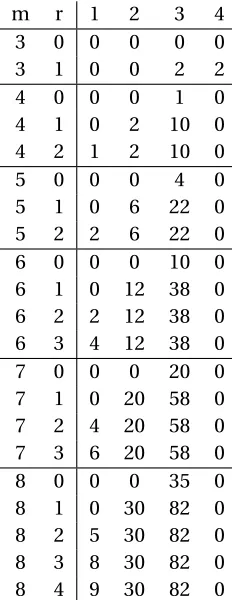
Table 2.4 The number of degree 1, 2, 3, and 4 generators form,r . . . 62
Table 4.1 Paired comparison matrix for HIV data . . . 92
Figure 1.1 Graph of the varietyV(y−x3)inR2. . . . 4
Figure 1.2 Graph of the varietyV(y−x3)inR3. . . . 4
Figure 1.3 Hasse diagram of the poset defined by all subsets of{x,y,z}ordered by set inclusion. . . 9
Figure 1.4 Visualization of permutation 2431 inS4. . . 11
Figure 1.5 Visualization of composition of the permutation 2431on the left with 3241 inS4 11
Figure 1.6 The graph of the probability density function for a Gaussian random variable Xwithµ=0,σ=1 . . . 17
Figure 2.1 The Cayley graph ofS4 . . . 32
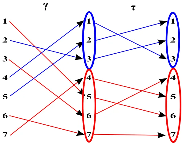
Figure 3.1 The composition ofτγwhenτis a direct sum, with disjoint subsets highlighted 71
Figure 3.2 The composition ofτγwhenτis a skew sum, with disjoint subsets highlighted 73
Figure 3.3 The composition of τγwhenτis a permutation consisting of contiguous blocks, with disjoint subsets highlighted . . . 78
Figure 3.4 The composition of τγwhenτis a permutation consisting of contiguous blocks, highlighting the permutation pattern of 123 inτγ. . . 79
Figure 4.1 Graphical representation of proposed model . . . 84
Figure 4.2 The mutations corresponding to variablesXi and the maximum likelihood poset proposed in[3]. . . 91
1
INTRODUCTION
with as well as examine their underlying structure from an algebraic and combinatorial perspective. Before we do, we examine the aspects of statistical models for ranked and partially ranked data in greater detail.
In this chapter, we introduce the underpinnings from algebraic geometry, combinatorics, and statistics which are used throughout the thesis. In Section 1.1, we will define the pertinent constructs from algebraic geometry, establish notation, and remind the reader of a few basic theorems from the field which will be used in this thesis. In Section 1.2, we provide the definitions from Combinatorics which will prove useful in this thesis. Furthermore, we explain the connection between ranked data and permutations, introduce theorems which will be useful while working with permutations and generating functions, and establish the notational conventions used for these concepts. In Section 1.3, we examine concepts from statistics to acquire the necessary background to understand the entirety of the thesis. This section is in no way intended to provide a comprehensive overview of all of statistics; as this is a thesis in Mathematics (as opposed to Statistics), we will be focusing only on the areas of statistics which will be relevant to the topics presented in this thesis. In Section 1.4, we will introduce some well known statistical models for ranked and partially ranked data and highlight some of the ways they have been used throughout various disciplines.
1.1
Background in Algebraic Geometry
In this thesis, we will make liberal use of the many tools afforded to us by algebraic geometry. We will cover some basic concepts of algebraic geometry which will be necessary for understanding the thesis. In order to do this, we first make explicit some of the notation we use as well as remind the reader of some important concepts in Algebraic Geometry. We letk denote a field,k[x1, . . . ,xn]denote the polynomials in variablesx1, . . . ,xnwith coefficients ink. We will often refer tokas the base field and shorten the notationk[x1, . . . ,xn]tok[x]in the places where it is clear thatxis short form ofx1, . . . ,xn. A nonzero polynomial
f = X
α1,...,αn
cα1,...,αnx
α1
1 · · ·xnαn cα1,...,αn∈k
which we say has degree (or total degree)d ifcα1,...,αn =0 wheneverα1+· · ·+αn>d andcα1,...,αn 6=0 for some indexα1+· · ·+αn=d. We will frequently denote the degree of a polynomialf as deg(f). We can then define the polynomial as homogeneousifcα1,...,αn=0 for allα1+· · ·+αn6=d. Whenever it is convenient to do so, we will use the multi-index notation
f =X
α
withα= (α1, . . . ,αn),cα=cα1,...,αn ∈k andxα=x
α1 1 · · ·x
αn
n and|α|=α1+· · ·+αn.
We will letPn,d ⊂k[x1, . . . ,xn]denote the vector subspace of polynomials of degree≤d. We know the monomials
xα=xα1 1 · · ·xαnn form a basis forPn,d. Thus, we know
dimPn,d = n+d
n
.
Furthermore, given distinct pointsp1, . . . ,pN ∈An(k), we letId(p1, . . . ,pN)be the vector space of polynomials of degree≤d which vanish at each of the pointsp1, . . . ,pN. We will also make use of some basic definitions found throughout the algebraic geometry literature. First, we define an affine space.
Definition 1.1.1. Given a fieldk and a positive integern, we define then-dimensionalaffine space
overkto be the set
An(k):={(a1, . . . ,an) | ai∈k}. We will sometimes denoteAn(k)simply askn.
The classic example of an affine space is the case wherek =R, in which case then-dimensional affine space would simply beRn.
Definition 1.1.2. GivenS⊂An(k), the number of conditions imposed bySon polynomials of degree ≤d is defined as
Cd(S):=dimPn,d−dimId(S).
Sis said toimpose independent conditions onPn,d ifCd(S) =|S|. Otherwise, we say itfails to impose
independent conditions.
Next we can define a hypersurface.
Definition 1.1.3. Given a fieldkand a polynomialf ∈k[x1, . . . ,xm]where deg(f) =d. We define the
hypersurfaceof degreed as V(f):=
(a1, . . . ,am)∈Am | f(a1, . . . ,am) =0 ⊂Am(k).
Figure 1.1Graph of the varietyV(y−x3)in
R2
Definition 1.1.4. Letk be a field and f1, . . . ,fs ∈k[x1, . . . ,xn]. Then theaffine varietydefined by f1, . . . ,fs is the set
V(f1, . . . ,fs):=(a1, . . . ,an)∈kn | fi(a1, . . . ,an) =0 for all 1≤i≤s .
We consider two basic examples.
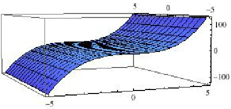
Example 1.1.5. Consider the variety inR2given by the single polynomialV(y−x3). We can use any computer algebra system to plot this variety. Here, we use Mathematica.
Note that if we were to consider the same variety inR3rather thanR2, the variety would look very different.
Figure 1.2Graph of the varietyV(y−x3)in
We assume the reader is familiar with ideals and monomial orderings and begin by defining the leading term of a polynomial.
Definition 1.1.6. Fix a monomial order onk[x1, . . . ,xn]and consider any nonzero polynomial f =X
α
cαxα.
Theleading termof f, denoted LT(f), is the termcαxαsuch thatxαis the largest monomial such that
cα6=0.
Recall that an ideal is calledhomogeneousif it is generated entirely by homogeneous polynomials.
Definition 1.1.7. GivenI ⊂k[x1, . . . ,xn]an ideal, we define theideal of leading terms LT(I):=〈LT(g) | g∈I〉
In a slight abuse of notation, if given a set of polynomialsG={g1, . . . ,gs}, we let LT(G):=
LT(gi) | gi∈G
This definition allows us to define the idea of a Gröbner basis.
Definition 1.1.8. Fix a monomial order and letI⊂k[x1, . . . ,xn]be an ideal. AGröbner basisforI is a set of nonzero polynomials{f1, . . . ,fs} ⊂I such that LT(f1), . . . , LT(fs)generate LT(I).
We know the following is true about Gröbner basis.
Theorem 1.1.9. Fix a monomial order and let I⊂k[x1, . . . ,xn]be an ideal. Let f1, . . . ,fs be a Gröbner basis for I . Then I=〈f1, . . . ,fs〉.
This well known result is just part of why Gröbner bases are such a powerful tool of algebraic geometry. It is also known that multivariate polynomial division using a Gröbner basis yields a unique remainder, thus answering the question posed by the ideal membership problem. It is well known that a Gröbner basis is not unique and depends largely on the choice of the monomial order.
We have already seen that an ideal can define a variety. We can also define the ideal defined by an affine variety.
Definition 1.1.10. LetV⊂An(k)be an affine variety. Then we define the setI(V)to be
I(V):=
More importantly,I(V)is an ideal (see, for example[10]). It is also true that an ideal is contained in the ideal of its variety.
Theorem 1.1.11. If f1, . . . ,fs∈k[x1, . . . , ,xn], then〈f1, . . . ,fs〉 ⊂I(V(f1, . . . ,fs)).
It should be noted that this containment is an equality only when〈f1, . . . ,fs〉is a radical ideal. The following propositions found in Hassett[22]are useful for understanding the relationship between a varieties generated by ideals and the ideals generated by that varieties.
Proposition 1.1.12. For every collection of polynomials F ={fj}j∈J ⊂k[x1, . . . ,xn]and each subset F0⊂F , we have that V(F0)⊃V(F).
Proposition 1.1.13. Given a collection of polynomials F={fj}j∈J⊂k[x1, . . . ,xn]generating an ideal I =〈fj〉j∈J, we have V(F) =V(I).
Proposition 1.1.14. For any subsets S0⊂S⊂An(k)we haveI(S0)⊂I(S).
We also know that an arbitrary intersection of varieties is a variety and a finite union of varieties is a variety.
Because we will make use of the pull-back of morphisms, we will define it here.
Definition 1.1.15. Choose coordinatesx1, . . . ,xnandy1, . . . ,ymonAn(k)andAm(k)respectively. Let φ:An(k)→Am(k)be a morphism given by the rule
φ(x1, . . . ,xn) = φ1(x1, . . .xn), . . . ,φm(x1, . . . ,xn)
whereφj∈k[x1, . . . ,xn]. Then for eachf ∈k[y1, . . . ,ym], thepull-backbyφis defined φ∗f =f ◦φ=f φ
1(x1, . . .xn), . . . ,φm(x1, . . . ,xn). We then have the ring homomorphism
φ∗:k[y
1, . . . ,ym] −→ k[x1, . . . ,xn] yj 7→φj(x1, . . . ,xn).
Furthermore,φ∗ has the propertyφ∗(c) =c for all constantsc ∈k and is therefore ak-algebra
homomorphism.
It is true that there is a natural correspondence between morphisms andk-algebra homomor-phisms (see, for instance,[22]).
Definition 1.1.16. Given a ringRand a collection of ideals{Ij}j∈J inR. Thesumof these ideals is the ideal
X
j∈J
Ij :=¦f1+· · ·+fs | fj ∈Ij for somej ©
In other words, the ideal consisting of all finite sums of elements each taken from one of theIj Before we define the join of ideals and the join of varieties, we will introduce some notation. We will let∆N denote the variety
∆N:={(t1, . . . ,tN) |t1+· · ·+tN=1} ⊂AN(k)
We also know that for every finite set of pointsS={p1, . . . ,pN} ⊂An(k), there is a morphism σS : ∆N→An
(t1, . . . ,tN)7→t1p1+. . . ,tNpN
where we add thepj as vectors inkn. The image is called theaffine span ofSinAn(k)and is denoted affspan(S). The following proposition can be found in[22].
Proposition 1.1.17. The set S={p1, . . . ,pN}imposes independent conditions on polynomials of degree ≤1if and only ifσSis injective. We say that S is inlinear general position.
We will use the definition presented by Sidman and Sullivant in[38].
Definition 1.1.18. Given a collection of idealsI1, . . . ,Ir ⊂k[x1, . . . ,xn]. ThejoinofI1, . . . ,Ir is the ideal
I1∗ · · · ∗Ir :=
I1(y1) +· · ·+Ir(yr) +〈xj− X
yi j | j ∈[n]〉 \ k[x]
whereyi is a new set of variablesyi = (yi1, . . . ,yi n)andIi(yi)denotes the ideal obtained from Ii by substituting the variableyi j for the variablexj. It should be noted that the large ideal in the parentheses is contained in the ringk[x,y1, . . . ,ym].
Definition 1.1.19. LetV1, . . . ,VN ⊂Anbe affine varieties. Thejoinof these varieties, denoted Join(V1, . . . , ,VN)⊂ An, is defined as the closure of the image
V1× · · · ×VN×∆N→An
There is a nice relationship between the join of two varieties and the variety of the join of those two ideals. In short, given to idealsI,J and considering their varietiesV(I),V(J), we know that the varietyV(I∗J)is the join of the varietiesV(I)andV(J). Geometrically, the join of two varietiesV,W is the union of all points which lie on a line which contains a point inV and a point inW. In other words, it is the union of all lines which pass throughV andW.
1.2
Background in Combinatorics
Throughout the thesis, we will make us of the notation[n]to denote the set{1, . . . ,n}.
Because we will be dealing extensively with partially ordered data, it will make sense to define a poset.
Definition 1.2.1. Apartially ordered set(orposet)Pis a set on which there is some binary relation≤ which satisfies the following properties:
1. For allx∈P,x≤x(reflexivity)
2. Ifx≤y andy≤x, thenx=y (anti-symmetry) 3. Ifx≤y andy≤z, thenx≤z (transitivity)
Within a posetP, we say that two itemsxandy arecomparableif eitherx≤y ory ≤x. If neither of these is true, we say the itemsx,y areincomparable. We will say that a posetPhas an element0 ifˆ there exists an element0ˆ∈Psuch that for allx∈P,0ˆ≤x. SimilarlyPhas an elementˆ1 if there exists an elementˆ1∈Psuch that for allx∈P,x≤1. Ifˆ s,t ∈P, then we sayt coverss(orsis covered byt) if s<t and there does not exists an elementr∈Psuch thats<r<t. It is known that a locally finite poset is completely determined by such cover relations. TheHasse diagramof a finite posetPis the graph whose vertices are elements ofPand whose edges are cover relations, where ifs<t then the vertext is drawn with higher vertical coordinate than that of the vertexs.
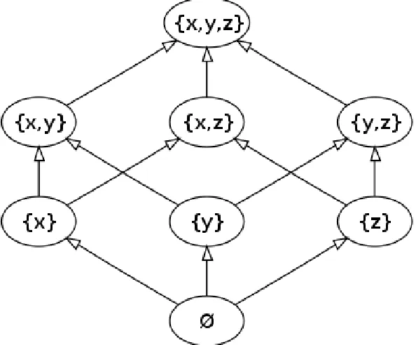
Example 1.2.2. As a standard example, we can create a poset out of the 2[n]subsets of any set[n]with
the order relation being the standard set inclusion (i.e.,S≤T in the poset ifS⊂T). We consider the set{x,y,z}and the poset consisting of all subsets of this set. We can visualize this poset by creating a Hasse diagram. The Hasse diagram for this poset can be found in Figure 1.3.
Figure 1.3Hasse diagram of the poset defined by all subsets of{x,y,z}ordered by set inclusion.
When dealing with ranked data, we will work with permutations rather than posets. We will now define the aspects of permutations we will use in this thesis. Recall that a permutationπ∈Sn is a bijective map from[n]to[n]. While there are different ways to denote a permutation, we will use one line notation exclusively. To remind the reader, any permutationπ∈Sncan be written asπ=π1· · ·πn which indicates the permutation mapsitoπi (again, bothi,πi∈[n]). We can define an inversion of a permutationπ=π1· · ·πnto be a pair(i,j)∈[n]×[n]such thati<jandπi> πj. Then we have the following
Definition 1.2.3. We denote the number of inversions of a permutationπ∈Snas inv(π)and therefore inv(π):=#
(i,j)∈[n]×[n]| i<j and π(i)> π(j) .
We know that for anyπ∈Sn, 0≤inv(π)≤ n2
reverse would yieldπ−1).
While we will denote a permutation in one line notation throughout the thesis, we will make use of permutation matrices. Given a permutationπ∈Snwithπ=π1· · ·πn, the permutation matrix ofπ, denotedMπ, will be then×nmatrix withMi,j =1 ifπj =i(i.e.π(j) =i) and 0 otherwise. Permutation matrices always have exactly one 1 entry in every row and column (i.e. they are elementary matrices), and are therefore always of full rank.
Example 1.2.4. Consider the permutationπ=2431∈S4. The permutation sends 1 to 2, 2 to 4, 3 to itself, and 4 to one, as demonstrated in Figure 1.4. Furthermore, we we can find the permutation matrix of 2431 and it will have the form
M2431=Mπ=
0 0 0 1 1 0 0 0 0 0 1 0 0 1 0 0
.
We know that a composition of permutations is the composition of the two bijective functions, so we examine a composition of permutations. Now suppose we consider the permutationσ=3241 with permutation matrix
M3241=Mσ=
0 0 0 1 0 1 0 0 1 0 0 0 0 0 1 0
.
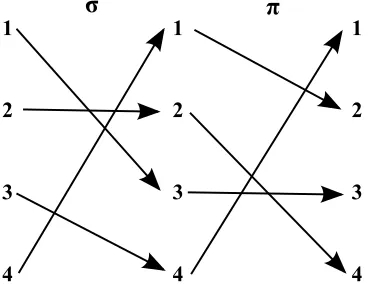
We know that the compositionπσwill apply the mappingσfirst and then apply the mappingπ. The result is that first 1 will map to 3 (viaσ) which will map to 3 (viaπ), 2 will map to 2 which will map to 4, etc., and the resulting composition will be the permutation 3412, as shown in Figure 1.5. The result can also be achieved by multiplying the permutation matrices:
MπMσ=
0 0 0 1 1 0 0 0 0 0 1 0 0 1 0 0
0 0 0 1 0 1 0 0 1 0 0 0 0 0 1 0
=
0 0 1 0 0 0 0 1 1 0 0 0 0 1 0 0
.
1
2
3
4
1
2
3
4
π(1)
=2
Figure 1.4Visualization of permutation 2431 inS4
1 2 3 4 1 2 3 4 1 2 3 4
σ
π
Figure 1.5Visualization of composition of the permutation 2431on the left with 3241 inS4
permutations which have one line notationεi=1· · ·i+1i· · ·n. For all permutationsπ∈Sn, we can writeπas a product of adjacent transpositions,Qiεji. If we were to think of permutation matrices, these adjacent transpositions would correspond to permutation matrices of the form
1 0 · · · 0 0 ...
..
. 0 1 ...
1 0 ..
. 1
... 0 0 · · · 0 1
The sign of a permutation can be defined in terms of the number of adjacent transpositions required to generate that permutations. If we letε1, . . . ,εn−1be then−1 adjacent transpositions which generate Sn. Then for anyπ∈Sn,π=εi1· · ·εik and we define thesign ofπis defined as
sgn(π):= (−1)k .
Permutations inSncan generally be thought of as a specific ordering of the set[n]. While every element of[n]is unique, we can extend the idea a permutation to be an ordering of a multiset. Recall that a multiset behaves in many ways like a set, with the exception that there can be repeated elements and elements that are repeated are indistinguishable from one another. For example,M={1, 1, 2, 3}is a multiset where both of the elements 1 are treated as identical.
Definition 1.2.5. LetMbe any multiset. LetSMdenote the set of permutations of the multisetM.
Example 1.2.6. Consider the multisetM={1, 1, 2}. Then we can list all the permutations ofM:
SM={112, 121, 211}. If we instead letM={1, 1, 2, 3}, we will have
SM={1123, 1213, 1231, 1132, 1312, 1321, 2113, 2131, 2311, 3112, 3121, 3211}.
Definition 1.2.7. The polynomial
1+q+q2+· · ·+qn−1=1−q n 1−q is denoted(n)and is called theq-analogue ofn.
Then we can define theq-analogue ofn! as
(n)!= (1)(2)· · ·(n) =1(1+q)(1+q+q2)· · ·(1+q+· · ·+qn−1).
Similarly, theq-analogue ofn choosek is
n k
= (n)! (n−k)!(k)!
then we let(n)!g(x)be theq-analogue ofn! evaluated whenq=g(x). That is
(n)!g(x)=f g(x).
Of course, we can extend this definition to theq-analogue ofnchoosek. That is
n
k
g(x)
= (n)!g(x) (n−k)!g(x)(k)!g(x)
Stanley shows that thatq-analogue ofn! can be thought of as a generating function[39].
Proposition 1.2.8(Stanley 2012). Letinv(ω)denote the number of inversions of the permutation ω∈Sn. Then
X
ω∈Sn
qinv(ω)= (1+q)(1+q+q2)· · ·(1+q+q2+· · ·+qn−1) = (n)! .
A similar result works for permutations of a multiset.
Proposition 1.2.9(Stanley 2012). Let M={1a1, . . . ,mam}be a multiset with cardinality n=a
1+· · ·+ am. Then
X
π∈SM
qinv(π) =
n a1, . . .am
.
We will also make use of a metric onSncalled Kendall’s tau metric. First, as we have mentioned, Sncan be generated by the adjacent transpositionsε1, . . . ,εn−1. That is, all permutationsπ∈Sncan be written as a product of adjacent transpositions,Q
iεji. We define the metric in the following way: given any two permutationsπ,σ∈Sn, the distance betweenπ,σis given by
d(π,σ) =inv(πσ−1).
We will also make use of the fact that the symmetric groupSnis a Coxeter group. We will assume the reader is familiar with Coxeter groups. We will define those concepts we will use in this thesis. One of the things we will use is a Bruhat order on the symmetric group. We will define the terms we will use when thinking ofSnas a Coxeter group.
way to writeωas a product of fewer thankadjacent transpositions. In this case, we say thelength of
ωisk. It is true for allπ∈Snthat the length ofπis the equal to d(π, id). Note that reduced expression are not in general unique.
We can now define the weak left Bruhat order onSn.
Definition 1.2.11. Consider the symmetric groupSnand recall that it is generated by the adjacent transpositionss1, . . . ,sn−1as defined above. The weak left (Bruhat) order onSnis the partial order on the groupSn with the relation≤which. for any two elementsπ,σ∈Sn, is defined asπ≤σif there exists a reduced expressionσ=si1· · ·sik such thatsi`si`+1· · ·sik =πwhere`is the length ofπ. That is, there is a reduced expression of forσwhose final substring is a reduced word forπ.
Finally, we know thatSnwith generators{s1, . . . ,sn−1}is a Coxeter group as well as a braid group. We will define braid moves here.
Definition 1.2.12. ConsiderSn generated by the adjacent transpositions{s1, . . . ,sn−1}. The relations sisj =sjsi for with|i−j|>1 andsisi+1si =si+1sisi+1fori,j ∈[n−1]hold in any Coxeter group, includingSn, and a substitution of these forms in a word is calledbraid moves(or sometimesbraid transformations). Not that because these are equalities, the word itself will not change due to a braid move; while the arrangement and frequency of the letters may change, the overall word will not.
Note that these relationships hold for any Coxeter group, includingSn.
1.3
Background in Statistics
Finally, we provide the background necessary to understand the majority of the statistical methods we use in this thesis. As a form of shorthand, we will denote Pr(A)to denote the probability of an eventA. We will use Pr(A B)to denote the probability of the intersection of two eventsAandB, i.e. Pr(A∩B) =Pr(A B).
First, we assume the reader is acquainted with basic probability theory, including the concepts of a sample space, events, and outcomes. We will also assume that the reader has a basic understanding of the axioms of a probability measure as well some of the more basic concepts of the concept of two events being disjoint within a space and partitions of a sample space. For a more complete background on statistics and probability, the reader can consult[43].
is a mapping
X:Ω−→R
that assigns a real numberX(ω)to each outcomeωin the state spaceΩ. We also must add that a random variable must be measurable in some way.
Example 1.3.1. If we flip a fair coin 5 times, we can letX(ω)denote the number of heads we observe in the sequenceω. Thus, forω=H H T H T,X(ω) =3.
We will stick to the convention that using a capital letterXwill denote a random variable, whereas a lower casexdenotes a particular sample or value of the random variableX.
Now we remind the reader of a probability function and a probability density function.
Definition 1.3.2. GivenX a discrete random variable (i.e.X can take on countably many values {x1,x2, . . .}). We define theprobability function(or sometimes aprobability mass function) forXby
fX(x) =Pr(X=x).
This is exactly what we would hope it would be: a function whose input is an outcome and whose output is the probability of observing said outcome. When the random variable in question is discrete, this is a perfectly good definition. The analogue for continuous random variables is a probability density function:
Definition 1.3.3. For a continuous random variableX, there exists a functionfX such that: 1. fX(x)≥0 for allx.
2. Z∞
−∞
fX(x)d x=1.
3. For everya≤b, Pr(a<X<b) = Zb
a
fX(x)d x. The functionfXis called theprobability density function.
As shorthand, we will generally usef(x)to denote the probability density function, and it should be clear from context which probability density function we are referring to. We may sometimes write R
f(x)d xto denoteR∞
−∞f(x)d x. It is important to remember that for continuous random variables,
we rely on integrals to obtain probabilities.
Definition 1.3.4. Given two eventsA,Bon a sample spaceΩwith any probability distribution. Then the two eventsAandBare said to beindependentif
Pr(A B) =Pr(A)Pr(B)
and we writeA⊥⊥B. A set of events{Ai | i∈I}is independent if
Pr
\
i∈J Ai
=
Y
i∈J Pr(Ai)
for every finite subsetJ ofI.
For the most part, we will assume two (or more) events are independent. Returning to our coin toss example, we usually would assume the two coin tosses are independent, which would reflect the fact that the coin has no memory of the first toss. We can also derive independence by verifying the definition and confirming that in fact Pr(A B) =Pr(A)Pr(B). For example, if we roll a fair 6-sided die twice, and let the eventA={2, 4, 6}represent the event we roll an even number and the event B={1, 2, 3, 4}represent that you roll a number less than 5. The we know thatA B={2, 4}and can compute Pr(A B) =2/6=1/3, as we know all outcomes are equally likely. We can also compute Pr(A) =3/6=1/2 and the Pr(B) =4/6=2/3 and verify that Pr(A)Pr(B) =1/2×2/3=1/3 and so Pr(A B) =Pr(A)Pr(B)and concludeA ⊥⊥B. In this thesis, we will assume events are independent rather than derive they are independent. Note that disjoint events with positive probability are not independent (as Pr(A B) =Pr(;) =0 and Pr(A), Pr(B)>0).
Independence of events can also be conditional on other events. Given an eventBwith Pr(B)>0, we can define the conditional probability of an eventAgivenB.
Definition 1.3.5. If Pr(B)>0, then theconditional probabilityofAgivenBis defined as
Pr(A|B) =Pr(A B) Pr(B)
that you have a brain freeze given you ate something cold is not 1.
Before we examine the statistical techniques we will use in the thesis, we define a statistical model:
Definition 1.3.6. Given a sample spaceΩ, astatistical modelis a setP of probability distributions on the sample spaceΩ.
In practice, a statistical model incorporates the set of assumptions germane to the generation the observed data from a larger population. A model represents the data-generating process, usually in extremely idealized forms.
Most statistical models that are used in practice are parametric models. Aparametric modelis a set of probability distributionsP that can be parameterized by a finite number of parameters. We introduce one of the most famous parametric models in the following example:
Example 1.3.7. If we assume that the gathered data comes from a univariate Gaussian (or Normal) distribution, then the model is
P =
f(x|µ,σ) = 1 σp2π exp
−1
2
x−µ σ
2
;µ∈R, σ2>0
.
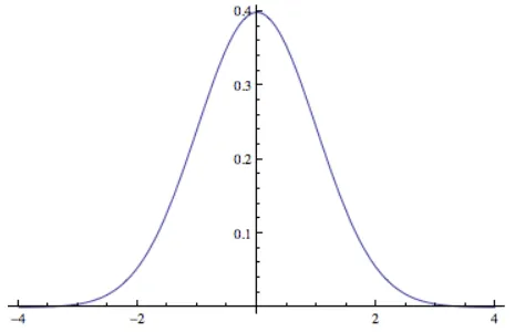
Here, we refer toµas the mean andσas the standard deviation. When a random variable follows this distribution, we refer to it as a Gaussian random variable (or Normal random variable). We denote that a random variableXfollows a Gaussian distribution with meanµand standard deviationσby X∼ N(µ,σ2). The graph for the probability density function for a Gaussian random variable with µ=0 andσ=1 is shown in Figure 1.6.
While it is true that there is a more general multivariate normal distribution, we will not use it within the scope of this thesis. In general, we denote that a random variableXis distributed to some parametric statistical modelPwith parametersθ with the notationX∼P(θ).
Statisticians use statistical inferences to analyze data. The two most dominant types of statistical inference:frequentist inferenceandBayesian inference. In this thesis, we are interested in recovering (or estimating) the parameters of a statistical model (as opposed to a probability density function or cumulative density function, for example). We will use both Bayesian and frequentist inference in Chapter 4 to do this. We will introduce the main idea of frequentist inference first.
Frequentist inference draws conclusions from sample data based on the frequency of that data. Statistical hypothesis testing and computation of confidence intervals are both frequentist techniques. We will make extensive use of maximum likelihood estimation throughout the thesis, which is another common frequentist technique.
Maximum likelihood estimation is a technique for estimating the parameters of a model when we do not have direct access to them. Since it is often the parameters of a statistical model that we are interested in sampling, this technique is rather common. During the general discussion of MLE techniques, we will refer to the set of parameters of a model asθ which comes from a parameter space Θ. In later sections, we will refer to parameters by their names rather than the generalθ.
Before we can truly talk about MLE, we must first introduce the likelihood function. This requires us to have some knowledge of random variables being independent and identically distributed (iid). This concept is basically summed up in its name: given random variablesX1, . . . ,Xn, we sayX1, . . . ,Xn areindependent and identically distributed(or iid) ifXi ⊥⊥Xj for alli6=jand each of theXi follows a single distribution with parameter setθi. Furthermore, for eachi, individual sample of the random variableXi are independent of one another.
Example 1.3.8. Consider a fair or unfair six-sided die. Rolls of that die are iid, regardless of whether it is fair, as each roll is independent of the others. That is, even if you roll a 6 five times in a row, rolling a 6 on the next roll has the same probability as it did on all the previous rolls. The same would apply for rolling multiple fair or unfair dice, provided there is a way to denote which die is which.
For a continuous random variable, we have the following:
Definition 1.3.9. Given a random variableXwith probability spaceΩand probability density function f(x). Theexpected value(ormeanorfirst moment) ofXis given by
E[X] = Z
Ω
x f(x)d x
assuming the integral is well defined.
Note that the expected value of a function requires integrating over the entire sample space. In cases where the sample space is more complicated, computing the expected value becomes more difficult. Later in this thesis, we will examine different methods to estimate the expected value of a random variable when computing the above integral is not straight-forward.
One fact worth noting at this point is if we haveg(X)a measurable function ofX, we can compute
E[g(x)] = Z
Ω
g(x)f(x)d x .
This fact is sometimes referred to as the Rule of the Lazy Statistician[43]. We are now ready to define the likelihood function:
Definition 1.3.10. LetX1, . . . ,Xn be iid with probability density function fi(Ai|θi). Thelikelihood
functionis defined by
Ln(θ|X) = n Y
i=1
fi(Xi|θi)
Thelog-likelihood functionis given by`n(θ) =logLn(θ|X).
In this thesis, we will only use the log-likelihood function. We note that the log-likelihood function is just the log of the joint density function, but we are treating it as a function of the parameterθ, as indicated by the notation. Sometimes, to make this even more explicit, we denote the log-likelihood function as`(θ|X)whereX= (X1, . . . ,Xn). It is worth noting that the log-likelihood function is not a density function, and therefore will not integrate to 1 (with respect toθ).
The definition of the MLE follows naturally
Definition 1.3.11. LetX1, . . . ,Xn be iid with probability density function fi(xi;θi). Themaximum
it usually is. A few notes about the MLE are that it is consistent–which means that it will converge to the true value of the parameter as sample sizes get larger and larger–and it is asymptotically normal. These results are contingent upon the model following certain well defined criteria; in this thesis, we will only use MLE in cases where the model meets the criteria necessary to guarantee that it is both consistent and asymptotically normal. We mention one theorem of note, which can be found in[43]:
Theorem 1.3.12. Letτ=g(θ)be a function ofθ. Letθnˆ be the MLE ofθ. Thenτˆ=g( ˆθn)is the MLE of τ.
Now we look at a simple example.
Example 1.3.13. Suppose we have a Gaussian random variableXwhose mean and standard deviation are unknown. We wish to find the values ofµ,σwhich maximize the log-likelihood function. Say we havenobservations. Letf(x|µ,σ) = 1
σp2π exp
−1 2
x−µ σ
2
. The log-likelihood function is
`(µ,σ | X) = n X
i=1 log
1 σp2π
+log e− 1 2
x(i)−µ σ
2!
=−nlog(σp2π) + n X
i=1 −1
2
x(i)−µ
σ 2
If we differentiate this equation with respect toµwe get d
dµ
−nlog(σ p
2π) + n X
i=1 −1
2
x(i)−µ
σ 2
= n X
i=1
x(i)−µ
σ2
When we set this equal to 0 we have
n X
i=1
x(i)−µ
σ2 =0 n
X
i=1 x(i)
!
−nµ=0 1
n n X
i=1
x(i)=µ
Similarly, if we were to differentiate with respect toσ: d
dσ
−nlog(σ p
2π) + n X
i=1 −1
2
x(i)−µ σ
2
=0 n
X
i=1
(x(i)−µ)2
σ3 =
n σ
1 n
n X
i=1
(x(i)−µ)2=σ2
and again we see that by definition, value ofσwhich maximizes the log-likelihood function is exactly the standard deviation of the sampledX(i). Thus, regardless of the number of samples taken, the maximum likelihood estimates for a univariate Gaussian random variable will be exactly the mean and the variance of the samples.
The Expectation-Maximization (EM) algorithm is an iterative method which inputs observed data to obtain the maximuma posterioriestimate for the parameters of a statistical model which has hidden (or latent or unobserved) variables. The algorithm has two steps, an Expectation step (E-step) and a Maximization step (M-step), hence its name. The EM algorithm has been applied to many different data sets and many different scenarios. We will focus on a rather straightforward application of the EM algorithm; we will assume the data is iid.
Before we give a formal outline for the EM algorithm, we will lay out the steps intuitively. First, we have observed dataY(1), . . . ,Y(N)which we collect, which will be associated with hidden variables X(1), . . . ,X(N). We will assume some initial estimateθ0for the true parametersθ. In the E step, we use the observed data to create a function for the expectation for the log-likelihood function`(θ|Y(·),X(·))
using the current estimate for the parameters. The M step then computes the value of the parameters that will maximize the function created in the E step. Then we repeat the E step using the new parameter estimation computed in the previous M step. The algorithm will produce a sequence of estimates for the parametersθi which converge to locally maximum likelihood parameters.
Before we formally give the EM algorithm, we will introduce some shorthand notation. When working with models where we have observed values of a random variableX, we will letX(i)denote the
ithobservation. If we want to refer to all observations of the variable, we useX(·). If ourX= (X
1, . . . ,Xn), thenX(i)= (X(i)
1 , . . . ,X
(i)
n )and we can refer to all observations of theith entry ofX asXi(·). We will sometimes refer to all observations ofX= (X1, . . . ,Xn)as simplyX.
dataY= (Y(1), . . . ,Y(N)) as well as unobserved dataX= (X(1), . . . ,X(N))with a vector of unknown
parametersθ and a log-likelihood function`(θ|Y,X) =p(Y,X|θ). The maximum likelihood estimate of the parameters is determined by the marginal likelihood of the observed data
`(θ |Y,X) =p(Y|θ) =X
X
p(Y,X|θ).
But because the hidden variableXcannot be observed, this quantity is almost always insoluble. This is where the EM algorithm can be used to recover a maximum likelihood estimate for the parameter.
Formally, the EM algorithm can be written as follows:
Algorithm 1.3.14. Given a statistical model which generates a set of observed dataY= (Y(1), . . . ,Y(N))
as well as unobserved dataX= (X(1), . . . ,X(N))with a vector of unknown parametersθ and a
log-likelihood function`(θ |Y,X)we initialize the algortihm with an initial value for the parameter vector θ0. Then fori=1, 2, . . ., repeat steps one and two below
1. (The E Step) Calculate the function:
K(θ|θi) =EX|Y,θi[`(θ |Y,X)]
where theθi and the observedYare fixed (θ is a variable). 2. Find the value ofθi+1which maximizesK(θ|θi). i.e.
θi+1=arg max
θ {K(θ|θ
i)}
The EM algorithm obtains an maximum likelihood estimate for the parameters of a model without computing`(θ |Y,X), but computing the expected valueEX|Y,θi[`(θ|Y,X)]can be equally difficult. We will see in Chapter 4 that we will need a way to estimate this expected value in order to make use of the EM algorithm. Still, the EM algorithm is a very powerful method for estimating parameters, especially in cases where the statistical model in question has hidden variables.
In the thesis which introduces the EM algorithm, Dempster, Laird, and Rubin modified the EM method to compute the maximuma posterioriestimates for Bayesian inference[11], making it a versatile tool in parameter estimation in both frequentist and Bayesian inference. For the model introduced in Chapter 4, we will be using the original EM algorithm along with methods for estimating the expected value in step 1 of Algorithm 1.3.14 to estimate the parameters of our model.
is collected. Because we are constantly updating the hypothesis, all Bayesian inference starts with a prior distribution on the value in question and seeks sample from the posterior distribution of that same value. This value is usually the true value of a parameter. Thus, we begin with an initial idea of that parameter might be by sampling from a prior distribution on that parameter. Then, we observe data, and finally, using that data and our parameter, we seek to sample from the posterior distribution on that parameter. We think of sampling from this posterior distribution as sampling from a distribution on the parameter of interest in light of the observed data.
We remind the reader of Bayes’ Theorem:
Theorem 1.3.15(Bayes’ Theorem). Let A,B be events in the sample space wherePr(B)>0. Then
Pr(A|B) =Pr(A) Pr(B|A) Pr(B)
This formulation of Bayes’ Theorem is for events in a sample space. If we have, instead, a sample space generated from random variables, we need to modify Bayes’ theorem in order for it to be useful. The modification for random variables follows from the original statement of Bayes’ theorem. We note that there are multiple formulations for Bayes’ theorem as regarded to random variables based on whether the random variables are continuous or discrete. We present the formulation which will be used most frequently in this thesis.
Theorem 1.3.16(Bayes’ Theorem for Random Variables). Given continuous random variables X,Y which generate a sample space. Let fX,fYdenote the probability density functions of X,Y respectively. Then we have
fX(x | Y =y) =
fY(y | X=x)fX(x) fY(y) We know from the law of total probability that
fY(y) =
Z ∞
−∞
fY(y | X=ξ)fX(ξ)dξ
improves as the number of steps increases. This is why MCMC algorithms are frequently employed in Bayesian techniques. Sampling from the posterior distribution is done by using a Markov chain, and taking enough of these samples allows for an accurate sampling from the posterior distribution of the parameters.
In Chapter 4, we will use a Bayesian technique known as a Gibbs sampler. Gibbs sampling is an MCMC algorithm used to obtain a sequence of observations which are approximated from the joint probability distribution of two or more random variables when direct sampling is difficult (or impossible). The sequence can be used to approximate the joint distribution, the marginal distribution of a single variable or a subset of the variables–including unknown parameters or hidden variables–or to compute integrals such as expected values. It is frequently used when the values of some of the variables are known, and therefore do not need to be sampled. It is a randomized algorithm, meaning it can be an alternative to deterministic algorithms, such as the EM algorithm. In its most basic form, Gibbs sampling is a special case of the Metropolis-Hastings algorithm.
Gibbs sampling is used in situations where the joint distribution of the random variables is not explicitly known or is difficult to sample directly, but the conditional distribution of each variable is known and is simple (or at the very least, easier) to sample from. The Gibbs sampling algorithm generates a sample from the distribution of each variable in turn, conditional on the current value of all the other variables. It has been shown that this sequence of samples is a Markov chain and the stationary distribution of this Markov chain is the joint distribution we are interested in.
The key idea behind Gibbs sampling is that if we are given a multivariate distribution, it is easier to sample from the conditional distribution than to marginalize by integrating over a joint distribution. The goal of a Gibbs sampler is to obtain a large number of samples of a random variable coming from a given joint distribution. The joint distribution, however, is either not explicitly known or not difficult to sample directly, so what a Gibbs sampler actually does is generate samples that approximate a joint distribution of all variables. Consider the most basic incarnation of the Gibbs sampler.
Algorithm 1.3.17(Gibbs Sampler). Given a random variableX= (x1, . . . ,xn). We wish to obtaink samples ofXfrom a joint distributionp(x1, . . . ,xn); denote theithsample asX(i)= (x1(i), . . . ,x
(i)
n ). Select some value ofX(0)as an initial value ofX. Then
1. To obtain thei+1stsample, sample each component variablexi+1
j (forj=1, . . . ,n) from the distribution of that variable conditional on all other variables using the most recent value of each of the other variables. In other words, if we are updating thejthcomponent, we update it according to the distributionp(xj | x1(i+1), . . . ,x(ji−+11),x(ji+)1, . . . ,xn(i))
When this kind of sampling takes place, we know that the samples approximate the joint distribu-tion on the variables, the expected value of any variable can be approximated by taking the average over all samples, and the marginal distribution over a subset of variables can be approximated by considering the samples for that subset of variables and ignoring variables not in the subset. The initial value can be determined randomly or by another algorithm, such as the EM algorithm.
When using Gibbs sampling, it is fairly common to ignore a number of samples taken from the beginning of the algorithm. This is commonly referred to as aburn in period. It is also common to only “observe" everynsamples after the burn in period. This prevents consecutive samples from being “trapped" in a particular part of the sample space, as well as ensures that each sample is sufficiently random. As an example, when running the Gibbs sampler in Chapter 4, we use a burn in value of 1000 (we discard the first 1000 full iterations of the Gibbs sampler) with 200 iterations between each sample afterward. In the context we use the Gibbs sampler in this paper, we know it converges to a true sampling of the posterior distribution[35].
Example 1.3.18. Suppose we have two Gaussian random variables,X,Y and our model dictates that both are distributed withµ=0,σ=1 with the added stipulation thatX≤Y. We can use Gibbs sampling to sample points from this space. Start with initial valuesX=Y =0. We first sampleX, noting thatX∼ N(0, 1). We know, however, thatX≤Y so we must preserve that relationship. There is any number of ways we could do this, but for now let’s use a truncated normal distribution (a distribution which behaves like a normal distribution but does not allow us to sample anyX>00). With a random sample we getX(1)=−1.2. Then we need to sampleY while preserving thatX≤Y.
Mathematically, we look for Pr(y | X=−1.2). Again we can use a truncated normal to do this, and might see that we getY(1)=−.45. When we look to sampleX(2), we use the value ofY(1)to ensure
that we preserve the relationshipX≤Y. Therefore, when we findp(x | Y =−.45)we might see that X(2)=−.82. We continue in this manner until we get the desired number of samples.
As mentioned before, the Gibbs sampler can also be used to estimate expected values and param-eter values. We will see more on this in Chapter 4.
1.4
Statistical Models for Ranked and Partially Ranked Data
model we consider in this thesis is based on the Mallows model. The Mallows model was originally proposed by Mallows in[29]in 1957. The paper contains many variations of statistical models for ranked data which come from different assumptions placed on the general model. The Mallows model is a location-scale model which assigns a probability to each permutation inSn. The probability the model assigns each permutation is based on two parameters: a center permutationκ∈Sn(which functions much like the mean of a normal distribution) and a parameterc ∈R+encoding spread
(which behaves very similarly to the standard deviation of a normal distribution). If we letpκ(π)
represent the probability of observing a permutationπ∈Snwhereκis the center permutation, we have
pκ(π) =e−cd(π,κ)−log(ψ(c))
wherec∈R+,e−logψ(c)behaves as a normalizing constant, and d(π,σ)is Kendall’s tau metric onSn,
defined by
d(π,σ) =inv(πσ−1) .
We will talk more about this metric as well as the Mallows model itself in Chapter 2.
A ranking can arise through a series of sequential comparisons where a single item is preferred to all remaining items and, after it is selected, is removed from all future comparisons. This concept lies at the core of the Plackett-Luce model. The Plackett-Luce model (P-L model) is a statistical model for ranked data which has been adapted for partially ranked data as well. The model stems from the idea that For fully ranked data, we havenitems to be ranked bykjudges and assume no ties, we have a set ofk observed rankings
{y(i)= (y1(i), . . . ,yn(i)) | i=1, . . . ,k}
whereyj(i)is the position (or rank) assigned to itemjby judgei. In other words, judgeiranks itemj in positionyj(i). This ranking is naturally associated with a permutationπ(i)=Snwhereπ(i)=y(i)
1 · · ·y
(i) n . The Plackett-Luce model (P-L model) is a distribution over all rankings which can be described entirely by a permutationσ. Thus, the probability assigned toσis not the probability of the permutation associated directly with a rankingy = (y1, . . . ,yn), but rather the probability assigned to the inverse of the permutation associated withy. The model has parameter vectorθ = (θ1, . . . ,θn)withθi ≥0 where θi is associated with itemi. This model assigns probability
Pr(σ |θ) = Y i=1,...,n
θσi Pn
j=iθσj .
Note that this is not the only formulation of this model.
the model has a posetP associated with it. Ifi<j is a relation of the posetP, then itemiis always ranked before itemj in the corresponding model. LetQbe the maximal chains of the posetP. The state space of this model is the setL(P)are the permutationsπ∈Snthat respect the relations ofP, i.e. they are the permutations which are linear extensions ofP. Note that this model’s state space is not all ofSn. The probability function can be obtained from the Plackett-Luce model for fully ranked data by normalizing over a subset ofSn(for more on this, see[41]. Then we see that for anyπ∈ L(P), the probability of observingπis given by
Pr(π | θ) = n−1 Y
i=1 1 Pi
j=1θπ(j)
for π∈ L(P) .
While we will not make use of the P-L model in this paper, several well known statistical tools can be used with the P-L model. The authors of[1]demonstrate how to use regression in a P-L model. Microsoft researchers Guiver and Snelson give an efficient method for inferring the parameters of P-L model in[21]. Mollica and Tardella develop methods for efficiently running the EM algorithm and a Gibbs sampler on a mixture of Plackett-Luce models[30]and use a mixture of P-L models to model epitope profiling[31]. The authors of[7]propose a Bayesian nonparametric extension of the P-L choice model capable of handling an infinite number of choice items.
Thurstonian models are a third class of statistical models for ranked data. Proposed in 1927, the Thurstonian model assumes that every item being ranked has an inherent, unobservable true value
[42]. The model observes rankings onnitems by a judge (or judges). The Thurstonian model assumes the each item is given a valueXi whereXi ∼ N(µi,σ2i). The meanµi is the true value of that item and σi is an unobservable parameter associated with the item. The ranking a judge assigns to the items depends entirely on the value ofXi’s–the ranking assigned to an itemiwill be #{j | Xj <Xiwhere j6=i}. Within the framework of this model, it is possible for the same judge to rank the same items in different ways. The notable aspects of this model assumes the value assigned during each ranking by each judge (where there are potentially multiple judges and multiple rankings from each judge) are continuous real number values which cannot be observed and these values are distributed according to a normal distribution.
used as methods for parameter estimation are developed and are made more efficient. In the sensory field, authors Bi and Kuesten claim that Torgerson’s method of triads has been avoided due to the fact that the Thurstonian model that is a part of the method and “there are no published tables or available computer software for applications of the method[4]." In their paper, the propose a Thurstonian model for a special case of Torgeson’s method of triads. Ennis and Rousseau develop a Thurstonian model for degree of differences methodology, a methodology where subjects are given pairs of samples and must indicate how different the are on at-point scale[16]. The model can be used in many discrimination, rating, and ranking methodologies. The authors of[9]propose and alternative to the two-Alternative Forced Choice (2-AFC) model in which participants are presented a pair of items and asked which is preferred where the response of “no preference" is allowed. They then detail ways to extract estimates and standard error of the parameters in this two-alternative choice model. Gianola and Simianer introduce a fully Bayesian method for quantitative genetic analysis of data consisting of ranks which are scored at a series of events or experiments[20]. The rank observed is assumed to reflect the order of values of some unobserved variable which is distributed normally, and is therefore another application of the Thurstonian model. We will talk about more applications of Thurstonian models as well as methods for estimating values of interest in a Thurstonian model in Chapter 4.
We seek to study these models from an algebraic and combinatorial point of view.
1.5
Outline of Thesis
2
THE MALLOWS MIXTURE MODEL
The Mallows model is a statistical model for ranked data which gives a closed form for computing the probability of observing a particular permutation inSn. It is a location scale model, much like the normal distribution, meaning the probability assigned to each permutation will decrease the further away it is from the “center" permutation. The Mallows model has been used in a number of different disciplines. Lebanon and Mao set up the framework for using the Mallows model specifically on permutations which are partition-preserving[26]. In this chapter, we build on this framework and examine a mixture of Mallows model. The interest in doing so comes in part from the work of Lebanon and Mao.
In this chapter, we introduce a mixture model based on a classic statistical model for ranked data, the Mallows model. The original model, proposed by Mallows[29], makes use of paired comparison techniques as well as Kendall’s tau metric on the symmetric group. The model is designed to be used for ranked data. That is, the observations are entire rankings on a set ofnitems. Because of this, it is natural to think of the observations as permutations inSn. In Section 2.1 we introduce and examine the vanishing ideal of the original Mallows model. In Section 2.2 we will introduce the Mallows mixture model which we analyze and characterize in later sections. In Section 2.3 we introduce theorems to completely describe all(i,j)pairs in{0, . . . , n2
degree in Section 2.4. Using the theorems for Section 2.3 and Section 2.4, we look at the vanishing ideal of the map of the Mallows mixture model in Section 2.5. In Section 2.6 we look at the number of generators of various degrees.
2.1
The Mallows Model
The original Mallows model was proposed by Mallows in 1957[29]. It is a location-scale model for ranked data for which uses paired comparisons to assign a probability to every possible ranking. Because the observed data points in this model are rankings onnitems, it is natural to think of these observations as permutations inSn. Thus, if we were to rank 4 items{1, 2, 3, 4}, the permutation 4132 is equivalent to the ranking where item 4 is ranked first, item 1 is ranked second, etc. The model has a center, much like a mean. That is, the closer a permutation is to the center, the more likely it will be observed. A well defined concept of “closeness" requires a metric onSn. We choose Kendall’s tau distance as our metric. Recall the symmetric group is generated by then−1 adjacent transposition of Sn. Under Kendall’s tau metric, the distance between any two permutations is the minimum number of adjacent transpositions necessary to compose with one of the permutations to transform it into the second. That is, d(π,σ) =inv(πσ−1). For instance, the distance between 3142 and 1243 is 2, as seen in Figure 2.1. The Cayley graph is a visualization of distance between elements ofSn.
This is just one way to describe Kendall’s tau distance, but it is the one we will use for the remainder of the paper. It should be noted that this is a right invariant metric. That is,
d(π,σ) =d(πτ,στ) ∀π,σ,τ∈Sn
Furthermore, for allπ,σ∈Sn, we know that 0≤d(π,σ)≤ n2
Under the Mallows model which is centered about the permutationκ, the probability of observing any probabilityπis exactly
pκ(π) =e−cd(π,κ)−log(ψ(c))
whereπ,κ∈Sn,c ∈R+, andψ(c)is the normalizing constant withψ(c) =Pπ∈Sne
−cd(π,κ). It will be useful to us to clean up this notation with a few simple substitutions. First, we note that since Kendall’s t