An approximation analysis of a shared buffer ATM switch under bursty arrivals

An

Approximation Analysis

of a

Shared Buffer ATM Switch

under

Bursty Arrivals

H.

Yamashita

H.

G.

Perras

S.

W.

Hong

Center for Communications and Signal Procesing

Department of Computer Science

North Carolina State University

TR-90/8

An App.roximatio.n Analysis of a Shared Buffer

ATM SWItch ArchItecture under Bursty Arrivals!

H. Yamashita", H.G.

Perros,

s.-

W.

Hong

Computer Science Department and

Center for Communication and Signal Processing North Carolina State University

Raleigh, NC 27695-8206, U.S.A.

Abstract: We present an approximation algorithm for the performance analysis of a shared buffer ATM switch architecture. The arrival process to each input port of the ATM switch is assumed to be bursty and it is modelled by an Interrupted Poisson Pro-cess. Comparisons against simulation showed that the approximation algorithm has a good error-level.

Keyword: ATM, shared buffer switch, bursty arrivals, Interrupted Poisson Process, queueing models, aggregation, approximation

1.

Introduction

One of the most promising solutions for Broadband ISDN is the Asynchronous Trans-fer Mode (ATM). Many ATM switch designs have been proposed, which provide a high throughput and a low cell loss probability. The most common design is based on mul-tistage interconnection networks. In this type of design, dedicated buffers may be at either the input ports or the output ports, or at both input and output ports. The input buffer switch has a simple architecture, but it achieves a very low throughput. On the other hand the output buffer switch is known to achieve the optimal throughput-delay performance[4].

Another switch architecture is the shared buffer switch, where all the output ports share the same buffer. This switch is based on the "Prelude" switch proposed by CNET, France[3]. This architecture is considered to achieve the optimal throughput-delay perfor-mance and requires less buffer memory than the output buffer switch mentioned above[4]. Few studies, however, have been carried out on the performance of this switch architec-ture. These studies are restricted to single queue analysis[1,5,6].

lSupported in part by DARPA under grant no. DAEA18-90-C-0039 and by the National Science Foundation under grant no. CCR-87-02258.

In this paper, we introduce an approximation algorithm for the performance analysis of the shared buffer switch. The approximation algorithm was developed assuming that the stream of arrivals to each input port is bursty and

it

is modelled by an Interrupted Poisson Process. In the following section, we describe the queueing model for the switch, and in section 3 we give the approximation algorithm. In section 4, we validate the ap-proximation algorithm by comparing it against simulation data. Finally, the conclusions are given in section 5.

2. Model Description

In the shared buffer switch architecture, the buffer memory is shared by all the switch output ports. An incoming cell destined for the output port i is stored in the shared buffer, and its address is stored in the address buffer. The mechanism to rou te the cell in the shared buffer to its output port can be implemented in various ways. The cells which have the same output port can be linked by the address chain pointer[5], or their addresses can be stored into a FIFO buffer which is dedicated to the specific output port[6]. A cell will be lost ifit arrives to find the shared buffer full or the address buffer full. The switch architecture is synchronized. Between two synchronization points any incoming cells that are in process of arriving at the input ports are written to the memory, and each output port transmits a cell (if there is one in its queue).

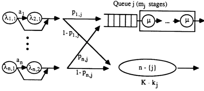
We model this system by the continuous time queueing model shown in figure 1. The queueing model consists of n single server queues, where n is the number of the input (or output) ports of the switch. Each server represents an output port. An incoming cell destined to output port i joins the ith queue. The total number of cells in all queues can not exceed M, the buffer size of the switch. A cell gets lost if it arrives at a time when the switch is full. It is possible that the total number of cells in each queue i may be limited to Ali where M,

<

M: In this study, we assume that Mi=M. However, the case where

M,

<

M

can be easily implemented.

Incoming links

Output ports

•

•

•

In the real system, the transmission time at each output port is constant. In view of this, we model the service time at a server by an Erlang distribution with r stages. All servers have the same service time distribution. Let Jj be the service rate at one

exponential stage. The arrival process to each input queue is assumed to be bursty and it is modelled by an Interrupted Poisson Process(IPP). That is, two separate exponentially distributed periods, an active period and a silence period, occur alternatively. During the active period, arrivals occur in a Poisson fashion. It can be shown that the time between two successive arrivals has a hyperexponential distribution with two stages, which in turn is equivalent to a Coxian distribution with two stages (hereafter referred to as C2

)[7].

In

view of this, we will assume that the arrival process to the ith input port is described by a

C2 distribution with parameters ~i,l ,~i,2' and 4i for i=1,2, ... ,n, where 4i is the probability

of going from stage 1 to stage 2. When a cell arrives at the ith input port, it chooses queue j with probability Pi,;, where

E;

Pi,j

==

1, i=I,2, ... n.

3.

The Approximation Algorit hrn

The approximation algorithm described in this paper is based on the notion of aggre-gation. For other applications of the aggregation technique to queueing systems with dedicated buffers or with shared buffers, the reader is refered to [2], [8], [9], [10], and [11]. The state of our model is described by the vector (~,m)=(wl,... ,Wn;ml, ... ,mn), where Wi, i==1,2, ,n, is the stages of the arrival process to the ith input port (wi=l or 2)

and mj, j=1,2, ,n, is the total number of stages to be completed by the cells in the jth queue. Let K be the total number of cells in the whole switch, and let Ie;, j=I,... ,n, be the number of cells in the jth queue. Then, we have

n n m.

K=Lk;=Lf-'l,

;=1 ;=1 r

O~K:=SM-l K==M

K==M

O~K:=SM-l

~i,l(K)

== {

~i,l'

0,

~i,2(K)

== {

~i,2'

0,

{

Il 1:::;mj:=SrM

JLj(mj)

==

0:

mj =

O.

Let P(w,m) be the steady state probability of the

st~te

(w,m). Furthermor:, for given w let WI and W

2 be the set of input ports which are in phase 1 and 2 respectively,

The global balance equations for the set (w, m) are as follows: where

r

a

l

is the least integer which is greater than or equal to a.

We now proceed to obtain the global balance equations for the above model. In order to simplify the notation, let us consider the following arrival rates and pseudo-service rates:

n

[L

{4iAi,1

+

(1 -

4i)Ai,I(K)}

+

L

Ai,2

+

~

JLj(mj)]P(w,m)

iEW

l iEW2 ,=1

+

+

+

n

~ ~_{L-J L-J}p'_I.J

·(1 -

a')'"_{I I.}IP(W_{- , -}m - re'?')_J

iEWl ;=1

-n

"L..J "p' .".L-J I,J I,

2P(W

-

+

e':'I , -m - re'?')J

iEWl j=l

-2:

"i.2(

K)P(

w

+

ei,

m)

iEWl

-n

(1)

+

2:

/LP(w,m

+

ej),

;=1

-where

ei

is the a-dimensional unit vector whose ith component equals to 1.

Note that with the exception of very simple cases, the solution of the system of linear equations (1) becomes intractable due to the very large number of states. In view of this, we analyze the queueing model under study approximately by analyzing each queue in isolation from the remaining queues. Let us focus on a particular queue j. The set of the remaining queues will be referred to by the symbol n-{j}. In order to analyze queue

j in isolation it is necessary to keep track of the number of stages left to be completed in the queue. Also, it is necessary to keep track of the total number of customers K in the whole system, so that one can decide whether an arriving cell can be admitted to the switch or not. However, in order to keep track of how K changes, it is necessary to know the rate at which cells depart from n-{j}. This departure rate is calculated using function

fj(K - k;) of the mean number of busy queues in n-{j}, where le; is the number of cells in queue j. This function is not known, and it is approximated iteratively as it

will

be described below.

•

•

•

Queuej (mj stages)

- - -

...

~

C

n-{j}::>

•

K - kj

Figure 2: Queueing structure of sub-system for queue j

(before aggregating the n arrival processes)

Thus, the switch is decomposed into n sub-systems, one per queue, &8 shown in

is very large due to the fact that each of the n arrival processes is represented by a C_{2 •} In order to reduce t.he dimensionality of each sub-system, we aggregate the n arrival processes into a single variable z which simply gives the number of the arrival processes which are in stage 2. As was mentioned above, the state of the n arrival processes is described by the vector (WI' W2, .•. ,wn ) . Due to the fact that each arrival process is independent from the

remaining processes, we have that p(W)=P(Wl)P(W2)···p(wn ) , where p(Wi) is simply the

probability tha.t the ith arrival process is in stage Wi. In view of this, p(1!) can be easily

obtained. Now, using the stationary probability vector p(1!.), we can easily aggregate the Markov chain of the n arrival processes to a Markov chain that gives all the transitions of variable z. In this way, we can significantly reduce the dimensionality of each sub-system shown in figure 2. Below, we present this approximation method in a more formal wa.y.

Let

Sz

be the set of states

W=(Wl, ...

,wn ) , where for each state there are exactly z

arrival processes which are in phase 2. As discussed above, we analyze queue j approxi-mately by keeping track of the number of input arrival processes which are in phase2

(z),

the number of stages to be completed by the cells in the jth queue

(mi)'

and the total number of cells in the whole switch (K). Denote by

Pj(z, mi, K)

the stationary joint prob-ability distribution of the state

(x,mj,K).

Pj(z,mj,

K)

is a marginal probability derived from P(w,rn) by

Performing this summation on equation

(1),

we get the aggregate balance equation as follows:

[:L

Prob{wlx,mj, K}{:L (ai'\i,l

+

(1 -

ai),\i,dK))

+

L:

'\i,2}

~ESI: iEWI iEW2

n K-r~l-l

+

p.(mj)+p.:L

:L

Prob{m/=rt+1I x,mj,k}]Pj(x,mj,K)

l=l,l~j t=1

L

Prob{wlx - 1,m;,K}

L

aiAi,IP;(Z - 1,m;,K)

~ES"_l ieWl

+

L

Prob{ wlz,

mj -

r,

K -

I}

L

Pi,j(l -

ai)'\i,lPj(Z, mj -

r,

K -

1)

~ES., iEWl

n

+

L

Prob{ wlz, mj, K - l}.L

L . Pi,l(l - ad'\i,l Pj(Z, mj, K -

1)

(2)

!!.ES. leWl'=1,I#J

+

'"'

Prob{wlz+1,mj-r,K-1} L

Pi,j'\i,2 Pj(z+1,mj-r,K-1)

L....J .w

y!E5.,+1 IE ,

n

+

L

Prob{wlz+1,mj,K-1}.L

L

.Pi,I'\i,2 Pj(z+1,m j,K-1)

ES leW21=1,I#J

y! .,+1

+

L

Prob{wlx

+

1,mj,

K} L

'\i,2(K)Pj(z

+

1,mj,

K)

EES.,+l iEW,

+

p,Pj(x,mj+l,K+vmj+l)

K-r~l

+

p.

i:

~

Prob(me=rt+1I z,mj,K+1)Pj(z,mj,K+1),

1=1,1#; t=l

for ~-O 1 n m

·=0

1 ... rM, and

K=O,l, ...

,M, where

{

I r~l = ~

-

,

,.

,.

IIm;+l - 0, r~

1

>

~.

Equation (2) is a set of linear equations with (n+l)(M+I)(Mr+2)/2 unknown prob-abilities Pj(x,mj,K). We note that these equations are exact if the correct values of the aggregate transition rates are used. However these aggregate transition rates contain two types of unknown conditional probabilities, namely

Prob{wlz,

mj,

K}

and

Prob{

m,

=

rt

+

l

le,

mj,

K}.

These probabilities are approximated as follows.

To begin with, we assume that the states of the input arrival processes do not depend on the total number of stages to he completed by a cell in service in the jth queue or on the total number of cells ill the whole switch, so that

where

and as reported in

[7],

Prob{wlz,mj,k}

~

Prob{wlz}

P(1Q)

P{Sz)'

L

P{w)

~ES.

(3)

In order to estimate the other type of conditional probabilities, we assume that a cell in queue

1(1

1=

j)

which is in service has the same proba.bility to be in any of the r Erlang stages. Moreover, the probability that a queue

1(1

-=I

i)

is empty is assumed to depend on the total number of cells in n-{j}, i.e,

n K-r~l-l

L

L

Prob{m,

=

rt

+

llz,mj,

K}

l=l,l~j f=l

t

1 -

Prob{Ie,

= Olz,mj,K}

l=l,l#j r

f.

1 -

Prob{Ie,

= OIK - lej }

j=l,l¥j r

fj(K - kj)/r

(4)

Here

/;(K - k

j ) is the mean number of non-empty queues in n-{j}, given that the number

of cells in n-{j} is K - kj , where kj is the number of cells in the ith queue.

/j{a)

satisfies

the following conditions.

1. /j(1)

=

1

3.

/;(a

+

1) -

fj{a)

>

/;(a

+

2) -

/;(a

+

1)

4.1;(0.)

<

min[n

-1,0]

1;(0.)

is not known and it is calculated as follows. Let 9,(0) be the mean number of non-empty queues in

n-{j}

when 0 cells arrive at the switch assuming that the service

time at each queue is infinite. Then we have

Clearly 1 ~ /i(O) ~ 9,(0), and therefore fj(o) can be approximated as

/,(o,{3)

=

1

+

{3[9;(0) - 1],

where

(5)

(6)

o:::;

{3 :::; 1.

Note that

9j(O)

satisfies the above four conditions, and so does

!i(a.,{J).

We estimate

/i(a) iteratively by adjusting f3 up and down accordingly inorder to meet the convergence criterion. Several different convergence criteria which must always hold can be condidered. In this study, the mean number of cells in the switch is used because it is computationally simple. The mean number of cells in the switch can be computed in the following two

different ways:

where

and

n M

~ ~

k

jPj

(1c; )

,=1 k,=1

1 n AI

- L L

KPj(K)

n

;=1K=1

n f"lej M

~ ~ ~ Pj(z,mj,K),

z=Omj=f"lcj-f"+1K=Ic,

(7)

(8)

n Kf"

Pj(K)

==

L

K ~

Pj(z, mj,

K).

z=O m, =0

E

1 must be equal to E2• Moreover, E1 - E2 is a monotonically increasing function of

{3 as well as of /;(

0).

We can, thus, decide whether the /;(

0)

is overestimated or un-derestimated depending on which mean is larger, and accordingly change

/;(0),

in order

to reduce the difference

E

1 and £2' Below, we summarize the proposed approximation

algorithm. The superscript s is used in order to denote an iteration number.

Algorithm

/3,-1+13,-1 ( )

L I M

d

i

1 2

b

step 1: 8=8+1,

13

M

= H 2 L and calculate

If

o,I3

M

lor 0= , ... , an J= , ,...,n y

using

(5)

and

(6).

step 2: Calculate conditonal probabilities by using (3) and (4), and then obtain

P/(z,mj, K)

for

j=1,2...

,n by solving numerically

(2).

This numerical solution is obtained by first set-ting up the underlying rate matrix and subsequently calculaset-ting the stationary vector of

P~(x,mj,

K)

using the

SOR

method.

step 3: Calculate

Ei

and

Ei

by using (7) and (8) respectively. step 4:

If

IE! -

E

21 ~ Ethen stop.

if E1 - E2

>

e then set

{3iI

==

{3M'

{3r

=

{3r-1

and go to step 1. if E1 - E2

<

- € then

{3il

==

{3H-1

,

{3L

==

(3M

and go to step 1.

4.

Validation

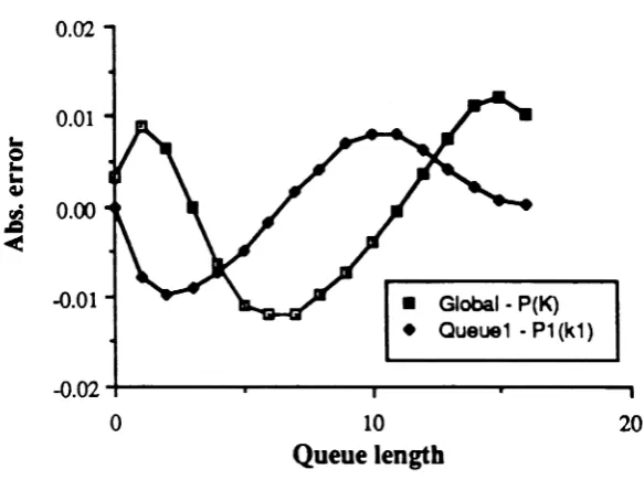
The approximation algorithm was implemented on a Cray super computer and it was used to analyze an 8x8shared buffer switch. The approximation results were compared against data obtained from a simulation model. Representative results are summarised in table.

1 to 5. Each table gives approximate and simulation results for the global queue-length distribution

P(K),

K==O,I, ...

,M,

and for the queue-length distribution Pt(lct

),lc

t=0,1...

,M

of queue 1, which is the most heavily utilized queue. Approximate and simulation results for the mean number of cells, m.q.l.,in the switch are also given. The absolute errors {or

P(K) and

Pt(k1 ) given in tables

1

to

5

have been plotted in figures

3

to

7

respectively.

The results have been obtained, assuming the following values for the 8 arrival processes.

Arrival process _{~i,l ~i,2} a

C

2 1 1.0025 0.0025 0.0025 200

2 1.0051 0.0050 0.0051 100

3 1.0064 0.0063 0.0063

80

4 1.0103 0.0101 0.0102 50 5 1.0130 0.0127 0.0128 40

6 1.0270 0.0256 0.0263 20 7 1.0586 0.0525 0.0554 10 8 1.7071 0.2929 0.4142 2

These values were obtained by assuming that each arrival process has an average arrival rate of 0.5, a peak arrival rate of 1, and a squared coefficient of variation of the interarrival time

C

2 _{as shown in the table above. The branching probabilities were as}

follows: Pi,t=0.25, Pi,2=0.2, Pi,3==0.18, Pi,4 = 0.12, Pi,s=O.I, Pi,8=0.08, Pi,7=0.05, Pi,8=O.02, i=1,2, ...,8. The service time distribution was assumed to be an

E

3 • The results in tables

1 to 5 were obtained by varying the total buffer space,

M,

and the service rate.

In general, the approximation algorithm gives good results. The approximate results for the queue-length distribution Pi(ki ) for each queue i seem to be slightly more accurate

than the global queue-length distribution P(K). The approximate results are not as good when the utilization of the output ports is very high (for instance, when the utilization of the output port

1,

which is the most heavily utilized, is more than

85%).

However, such

5. Conclusion

In this paper we presented an approximation algorithm for the analysis of the shared buffer ATM switch architecture under the assumption of bursty arrivals. Comparisons with simulation results showed that the approximation algorithm has good accuracy. This algorithm can be extended to the case where the bursty arrivals are also correlated. An-other possible extension is the analysis of the discrete-time version of the queueing model studied in this paper. These two extensions will be considered in our future work.

References

[1] P. Boyer, M. Lehnert and P. Kuhn, Queueing in an ATM basic switch element, Tech-nical Report, CNET-123-030-CD-CC, CNET (1988).

(2)

A.

Brandwajn and Y.-L.Jow, An Approximation Method for Tandem Queues with Blocking, Opere Res. 36 (1988) 73-83.

[3] M. Devault, J. Cochennec, and M. Servel, The "Prelude" ATD Experiment:

Assess-ments and Future Prospects,

IEEE J.

SAC, 6

(1988)

1528-1537.

[4]

M. Hluchyj and

M.

Karol, Queueing in High-Performance Packet Switching,

IEEE J.

SAC,6 (1988) 1587-1597.

[5] H. Kuwahara, N. Endo, M. Ogino and T. Kozaki, A Shared Buffer Memory Switch for an ATM Exchange, Proc. ICC'89, (1989),118-122.

[6] H. Lee, K. Kook, C. Rim, K. Jun, and S. Lim, A Limited Shared Output Buffer Switch for ATM, Fourth Int. Conf. on Data Communication Systems and Their Performance, Barcelona, June (1990), 163-179.

[7]

H.G.

Perros and

R.

Onvural, On the Superposition of Arrival Processes for Voice and Data, Fourth Int. Conf. on Data Communication Systems and Their Performance, Barcelona, June (1990), 341-357.

[8] P.J.

Schweitzer and

T. Altiok,

Aggregate Modelling of Tandem Queues without

In-termediate Buffers, in: Perros and Altiok, eds., Queueing Neiuiork« with Blocking (North Holland, 1989) 47-72.

[9] Y. Takahashi, A

New Type Aggregation Method for Large Markov

Chains

and Its Application to Queueing Networks, in: Akiyama, ed., Teletraffic Issues in an Advanced

Information Society, ITC-11 (Elsevier,1985) 490-494.

[10]

Y. Takahashi,

Aggregate Approximation for Acyclic Queueing Networks with Com-munication Blocking, in: Petros and Altiok, eds., Queueing Networks with Blocking(North

IIolland, 1989) 33-46.

K P(K) k1 PI(k1 )

approx. simul. approx. simul.

0 .1363 .1252±.OO32 0 .5202 .5116±.OO42

1 .1983 .1922±.0024 1 .2748 .2724±.0013

2 .1983 .1949±.0013 2 .1219 .1233±.OOI5

3 .1634 .1626±.0011 3 .0520 .0548±.OOll

4 .1195 .1219± .00 13 4 .0210 .0239±.OOO7

5 .0808 .0859±.OO14 5 .0075 .OO98±.OOO4

6 .0517 .0579±.0012 6 .0021 .0033±.OOO2

7 .0320 .0372±.0010 7 .0004 .OOO9±.OOOl

8 .0199 .0221±.OOO7 8 .0 .OOOI±.O

m.q.l 2.68 2.77

Table 1: Approximate and simulation results for P(K) and Pl(k_{1 )}

buffer size=8, service rate=2.0

0.01

...

0.00

0

...

...

QJ ~

~

<

-0.01

• Global· P(K)

• Queue1· P1(k1)

10

8

4 6

Queue length

2

-0.02-+---.---.--~--..--,.--r----.--""""---,,,,,---,

o

K P(K)

k

t

r.

(kt )

approx. simul. approz. simul.

0 .1299 .1273±.OO29 0 .5004 .5010±.OO39 1 .1860 .1903±.OO24 1 .2641 .2623±.OOO9 2 .187.4 .1888±.OO12 2 .1206 .1184±.OOI1 3 .1572 .1539±.OOO8 3 .0564 .0552±.OOO9 4 .1178 .1128±.OOO9 4 .0278 .0275±.OOO7 5 .0818 .0776±.OOI0 5 .0143 .0147±.OO06

6 .0539 .0517±.OOO9 6 .0076 .OO84±.OOO5 7 .0341 .0338±.OOO8 7 .0042 .OO50±.OOO3 8 .0211 .0219±.OOO7 8 .0023 .OO31±.OOO3 9 .0128 .O144±.OOO6 9 .0012 .OO20±.OOO2 10 .0076 .OO96±.OOO4 10 .0006 .OOI2±.OOOl 11 .0045 .0064±.OOO3 11 .0003 .OOO7±.OOOl

12

.0026 .OO44±.OOO3 12 .0001 .0004

±

.0001 13 .0015 .O030±.OOO2 13 .0001 .OOO2±.O

14

.0009 .OO21±.OOOl 14

.0

.OOOl±.O

15 .0005 .OO14±.OOOI 15 .0 .0 ±.O 16 .0003 .OO09±.OOOl 16 .0 .0 ±.O

m.q.l 2.99 3.04

Table 2: Approximate and simulation results for P(K) and Pt(kt)

buffer size=16, service rate=2.0

0.006

0.004 .

0.002

s-f

-0.000

..

~

.!

-0.002

<

-0.004

• Global - P(K) • Queue 1- P1 (k1)

-0.006

o

10

Queue lengb

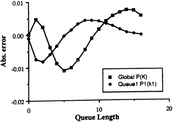
Figure 4: Absolute errors for the results in table 2

K P(K) kl PI

('I)

approx. sirnul. approx. simul. 0 .0445 .0478±.0025 0 .2719 .2719±.OO55 1 .0704 .0792±.OO26 1 .2033 .1954±.OO21 2 .0879 .0944±.OO20 2 .1389 .1291±.OOI1 3 .0956 .0955±.OO13 3 .0995 .0905±.OO13 4 .0956 .0892±.OOO8 4 .0752 .0677±.OOI2

5 .0906 .O799±.OOO8 5 .0587 .O538±.OO12 6 .0827 .O705±.0009 6 .0481 .0444±.OOll

7 .0737 .0620±.OOO9 7 .0357 .O372±.OOO8 8 .0647 .0548±.OOO8 8 .0267 .O308±.OOO9 9 .0563 .0490±.OOO8 9 .0188 .O256±.OOO9 10 .0488 .O447±.OOO7 10 .0123 .O201±.0009

11 .0423 .O418±.OOO8 11 .0071 .O149±.OOO8

12 .0368 .0403±.OOO7 12 .0036 .OO97±.OOO7 13 .0322 .O396±.OOO8 13 .0015 .OO55±.~

14 .0284 .0393±.OOlO 14 .0005 .OO25±.OOO2 15 .0256 .0380±.OO11 15 .0001 .OOO8±.OOOl 16 .0238 .0338±.OOI2 16 .0 .OOOl±.O m.q.l 6.42 6.62

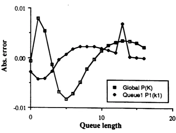
Table 3: Approximate and simulation result. Cor P(K) and PI(i1 )

buffer size=16, service rate=1.3

0.02

0.01

...

0

...

...

QJ

fI3 0.00

.c

<

-0.01

•

Global • P(K)

•

Queue1 • P1(k1)

20

10

Queue length

0.02. . . . . . . ... . . .

-o

K P(K)

k

1 Pt(kt )

approx. simul. approx. simul.

0 .0638 .0638±.0020 0 .3453 .3442±.0044

1 .1030 .1078±.OO21 1 .2378 .2304±.OOI4

2 .1239 .1263±.0017 2 .1458 .1377±.OOII 3 .1271 .1233±.OO13 3 .0920 .0860±.OOI1

4 .1182 .1094±.OO09 4 .0607 .O573±.OOlO 5 .1028 .O920±.OOO7 5 .0411 .O407±.OOO8 6 .0854 .O754±.OO07 6 .0282 .O297±.OOO8 7 .0686 .O610±.OOO8 7 .0191 .0224±.OOO7 8 .0539 .O494±.OOO8 8 .0127 .O170±.OOO7

9 .0416 .0405±.OOO8 9 .0081 .O124±.0006 10 .0318 .O334±.OO08 10 .0048 .0089±.OOO5 11 .0240 .O281±.OOO7 11 .0026 .0061±.0004

12 .0181 .0239±.OOO7 12 .0012 .OO39± .0003 13 .0136 .O205±.OOO6 13 .0005 .OO21±.OOO2 14 .0102 .0179±.OOO6 14 .0002 .OOlO±.OOOI 15 .0778 .OI52±.OO06

15

.0 .0000±.OOOl 16 .0061 .0120±.0005 16 .0 .0 ±.O m.q.l 4.92 5.14

Table 4: Approximate and simulation result, for P(K) and Pt('l)

buffer size=16, service rate=1.5

0.01

.. 0.00

e

..

~

.!

<

_-0.01

• GIobaJ P(K)

• Queue1 P1 (k1)

20

10

Queue Length

-0.02

-1----....---.,---....---,

o

K P(K)

'I

Pl(kl ) approx. simul, approx. slmul.

0 .0871 .0864±.OO28 0 .4157 .4129±.OO56 1 .1337 .1416±.OO28 1 .2566 .2513±.OO16

2 .1504 .155S±.OO20 2 .1383 .1341±.OOll 3 .1435 .1421±.OOI3 3 .0769 .0142±.OO11 4 .1236 .1168±.OOO7 4 .0449 .O445±.OO10

5 .0994 .O911±.OOO9 5 .0272 .O279±.0009

6 .0761 .0689±.OOI0 6 .0168 .OI85±.OOO8

7 .0563 .0514±.OO11 7 .0104 .OI26±.OOO7

8 .0406 .0383±.OOll 8 .0064 .0087±.0005

9 .0288 .O285±.OOO9 9 .0038 .0060±.0004 10 .0202 .0216±.OOOS 10 .0021 .0040±.OOO4

11 .0140 .O165±.OOO7 11 .0011 .OO26±.OOO3 12 .0096 .0127±.OOO6 12 .0005 .OOI5±.0002

13 .0066 .OlOO±.OOO6 13 .0002 .0007±.OOOl 14 .0046 .OO79±.OOO5 14 .0001 .0000±.OOOl

15 .0031 .OO61±.OOO4 15 .0 .OOOI±.O 16 .0022 .OO43±.OOO3 16 .0 .0 ±.O

m.q.l 4.00 4.09

Table 5: Approximate and simulation results (or P(K) and

PI(i

_{1 )}

buffer size=16, service rate=1.7

0.01

s-f:

...

~

,J. 0.00

.s

-e

• Global P(K) • Queue1 P1 (k1)

20

10

Queue length

-0.01.,....---....---~--~...- - - .

o