Approximate Analysis of a
Shared-Medium
A1~M
Switch Under Bursty
Arrivals and Nonuniform Destinations
,... ,.:n~;~) '-_~ 9
Atef
o.
Zaghloul
Center for Communications and Signal
Processing
Department of Computer Science
North Carolina State University
j/(j)IJJ
III
7~7:A
'l3/0-11{-93/2
Approximate Analysis of a Shared-Medium ATM Switch
under Bursty Arrivals and Nonuniform Destinations
Atef
o.
Zaghloul 1 and Harry G. Perros 21 IBM Corporation Departme nt C 15 RTP, N.C. 27709
USA
2 Department of Computer Science, and
Center for Communications and Signal Processing North Carolina State University
Raleigh, NC 27695-8206
USA
Abstract
In this paper, we present an approximate analysis of a generic shared-medium A TM switch with input and
output queueing. Input traffic is assumed to be bursty and is modelled by an Interrupted Bernoulli Process
(IBP). Three different bus service policies are analyzed: Time Division Multiplexing (TDA1), Cyclic, and
Random. The output links may have constant or geometric service time. The analysis is based on the notion
of decomposition whereby the switch is decomposed into smaller sub-systems. First, each input queue is
ana-lyzedin isolation after we modify its service process. Subsequently, the shared medium is analyzed as a
sepa-rate sub-system utilizing the output process of each input queue. Finally, each output queue is analyzed in
isolation. The results from the individual sub-systems are combined together through an iterative scheme.
This method permits realistic system characteristics such as limited buffer size, asymmetric load conditions,
and nonuniform destinations to be taken into consideration in the analysis. The model' s accuracy is verified
1.0
IntroductionThe Asynchronous Transfer Mode (ATM) is the adopted transfer mode solution for broadband ISDN.
ATM must be capable of efficiently multiplexing a large number of highly bursty sources, such as voice,
video, and large file transfer. As a result, there is an increasing interest in the performance analysis of ATM
based networks and in particular in ATM switches. There are severalATM switch architectures that have
been proposed recently in the literature (see for instance Cidon et al [1], and Turner [15]). ATM switch
architectures can beclassified into three classes: shared-memory, shared-medium, and space-division. Tobagi
[13] gives a detailed review of the different switch architectures and their implementation issues. In this
study, we are interested in the analysis of the shared-medium architecture. In a shared-medium switch, all
packets arrivingon the input linksarerouted to the output links overacommon high-speed mediumsuchas
a parallel bus. Each of the output links is capable of receiving all packets transmitted on the bus. The
PARIS system described by Cidon et al [1] and the ATOM switch proposed by Suzuki et al [11J, are two
examples of such a switch architecture. One of the main advantages of the shared-medium architecture is the
simplicity with which the multicast function is achieved since a transmitted packet over the shared-medium
can be received by all output links simultaneously. Thus, the need to send multiple copies is eliminated.
Also, priority among input links can be easily implemented within the bus arbitration policy. A
shared-medium packet switch can provide packet queueing at the input links, the output links, or both the input
and the output links (see Karol etal [6J and Pattavina [9J).
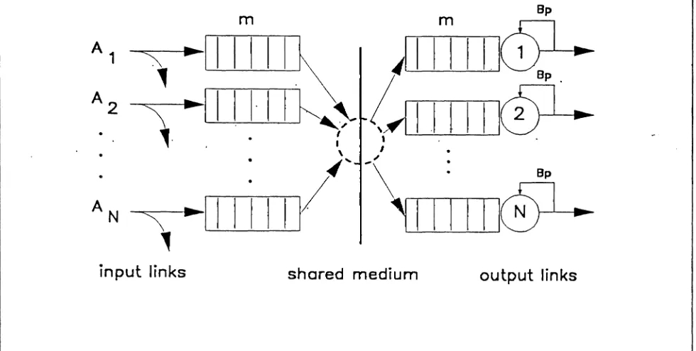
A queueing model of a generic shared-medium packet switch with input and output queueing is shown in
figure I. The input queues are attached to the shared bus and contend for access when they have one or
more packets to transmit. The order in which input queues are served is determined by the bus service
policy. In order to model such a system accurately, it is essential to take into consideration system
charac-teristics such as finite buffer capacities. bursty input traffic, nonsymmetric load conditions, and nonuniform
destinations. Cells arriving to a full input queue willbe lost. Furthermore, ifone of the output queues is
full, the flow of customers destined to it may be momentarily stopped. This situation is commonly referred
obtain. As a result, such queueing networks are typically analyzed approximately usmg the notion of
decomposition.
In this paper, we analyze the shared-medium switch shown in figure 1 under three bus service policies: Time
division multiplexing (TOM), Cyclic, and Random selection. The switch is analyzed approximately using
the notion of decomposition. First, each input queue is analyzed in isolation after we modify its service
process. Next, we analyze the shared bus as a separate sub-system utilizing the departure process from each
input queue. Finally, we analyze each output queue in isolation. Each sub-system is analyzed numerically as
a Markov chain. The results from individual sub-systems are combined together through the means of an
iterative algorithm. The accuracy of the approximation algorithm is verified via simulation.
The shared-medium switch, under cyclic and random selection bus service policies, can be viewed as a finite
capacity discrete-time polling system with blocking. The literature contains hundreds of papers on the
subject of polling systems (see Takagi [12]). However, most of the studies reported were for one-message
buffer systems or infinite buffer systems. Very few papers have dealt with finite buffer polling systems in
discrete-time or in continuous-time. Jou, Nillson, and Lai [5] analyzed a discrete-time polling system with
finite buffer capacity under bursty arrival process. Their approach gives an upper bound for the cell loss
probability. Tran-Gia [14J gives an approximate algorithm for polling systems with finite capacity and
non-exhaustive service. The analysis is based on the technique of the imbedded Markov chain and the evaluation
of discrete convolution operations taking advantage of fast convolution algorithms, e.g., the Fast Fourier
Transform. Ibe and Trivedi [4] considered finite-population and finite-capacity polling systems. Generalized
stochastic Petri nets are used to describe the system. The major drawback of this method is the large state
space of the system. Ganz and Chlamtac [2] presented an approximate solution to slotted communication
systems in continuous time with finite population and finite buffer capacity. Similarly, very little has been
reported in the literature on discrete-time queueing networks with blocking. Gershwin [3] analyzed a
discrete-time queueing network with blocking that represents a synchronized production assembly system. It
is often referred to as the transfer line model. The transfer line model has been analyzed by decomposing the
network to sub-systems each consisting of two successive servers and the buffer in-between. Recently,
Morris and Perros [7] developed an approximation algorithm for the analysis of a buffered Banyan ATM
for the analysis of multi-stage interconnection networks can be found in [7]. A sub-system of this switch
was analyzed approximately in [16]. See Perros [10] for a comprehensive review of queueing networks with
blocking.
The paper is organized as follows. In section 2, a description of the system under study is presented.
Section 3covers the analysis of the three sub-systems. Numerical results are presented and compared against
simulation results in section 4. Finally, conclusions are given in section5.
2.0
The Queueing model under studyIn this paper, we consider a single-stage N x N shared-medium switch with queue size (input and output)
equal to m as shown in figure 1. Cells may be queued before switching at the inputs, ifthe output queue is
full, as well as after switching at the outputs. A cell at the top of input queue i is destined for output queue
N
j with probability dij, where ~dij'
=
1, i=
1, 2, ... , N. Each input queue containing one or more packetsj = l
arbitrates for the bus by activating the bus-request signal. A bus arbiter is used to select the input queue to
be served next according to the bus service policy. Once an input queue has been granted the bus, only one
cell is forwarded to its destination output buffer. If the output buffer is full, then the cell will be blocked.
The blocked cell remain at the top of its input queue until the queue is granted the bus again. At that time,
the cellwillbe forwarded to output queue j with probability dij.
The bus bandwidth is N times the speed ofa single input link, where N is the number of input links. The
arrival process to each input queue is slotted, with a slot size equal to the transmission time ofan ATM cell.
The bus is also slotted, with a slot size equal to liN of the transmission time ofan ATM cell. For instance,
if N
=
6, then there arc 6 bus slots within the boundary ofeach arrival slot as shown in figure 2. Threedifferent bus service policies are considered in this paper: Time Division Multiplexing (TOM), cyclic order,
and random selection. These service policies are described in detail in section 3.1. We assume zero
switch-over time which means that when the bus completes serving the current queue, it switches instantaneously
and starts serving the next queue. This is normally accomplished by separating the control signals, which are
arbi-tration for the bus to be performed in parallel to data transmission; thus, justifying the zero switch-over
assumption. Finally, the service time of each output link consists of n arrival slots, where n is geometrically
distributed with parameterB; The servers of the N output links are synchronized. That is, they all begin and
end a slot at the same time.
The arrival process to each of the input queues is assumed to be bursty and it is modelled by an Interrupted
Bernoulli Process (IBP). That is, the incominglink into an input queue is slotted, Each slot is long enough
to contain one cell. An arriving slot mayor may not contain a cell. In an IBP, we have a geometrically
distributed period during which no arrivals occur (idle state), followed by a geometrically distributed period
during which arrivals occur in a Bernoulli fashion (active state). Given that the process isin the active state
at slot t, it will remain in the active state during the next slot t
+
1with probability P. or it will change to theidle state with probability I-p.
If
the process is in the idle state at slot t, it will remain in the idle stateduring the next slot t
+
1 with probability q, or itwill change to the active state with probability l-q. Duringthe active state, a slot contains a cell with probability C1.. The quantity C1. is also known as the peak
band-width, i.e., the rate of arrivals during the active period. In [8], the average arrival rate, i.e., the probability
that any slot contains a cell, is calculated as:
a(1 - q)
p=
2-p-q
and the squared coefficient of variation, 0, of the time between successive arrivals is
c
2=1
+a[
(l-P)(P+~)
-IJ .
(2 - p - q)
Because of the finite buffer space at the input links, a cell arriving to a full input queue is lost. However,
once a cell has been received, it will not be lost within the switch. In this paper, we assume that a is equal
3.0
The analysisThe shared-medium switch described in the previous section is analyzed approximately by decomposing it
into smaller sub-systems. First, each input queue is analyzed separately after we revise its service process.
This revised service process which we willcall the effective service time consists of three components. The
possible delay due to bus contention, the actual bus transmission time (one bus slot), and the blocking delay
due to a full destination queue. Having analyzed each input queue, we proceed to analyze a sub-system that
represents the bus. The arrival process to this bus sub-system from each input queue i is approximated by
an IBP, is obtained from the attempted departure process of input queue i. Finally, each output queue is
analyzed in isolation. The attempted departure process out of the bus sub-system serves as the input process
for the output queues.
Each sub-system is analyzed numerically as a Markov chain. However, in order to analyze each sub-system,
information is needed from the other sub-systems. This information is updated through an iterative scheme.
The algorithm iterates until convergence. Sections 3.1 and 3.2 describe the analysis of the input queues and
the bus respectively. The analysis of the output queues is presented in section 3.3. Finally, a summary of
the algorithm is given in section 3.4.
3.1
Analysis of the input queuesAs stated earlier, each input queue is analyzed in isolation after we revise its service process. This revised
service process is described in sections 3.1.1, 3.1.2, and 3.1.3 for TDM, Cyclic, and Random selection
poli-cies respectively. In section 3.1.4 \VC derive the cell loss probabilities for the input links.
3.1.1 TOM
Time Division Multiplexing (TDlvl) is the simplest bus allocation scheme. In TOM each bus sloti is
preas-signed to input queue i. Each input queue is only allowed to transmit during the bus slot aspreas-signed to it. If
assignments follow a predetermined pattern that repeats itself periodically as shown in figure 2. Each such
period is called a bus cycle. Once, a cell reaches the head of an input queue, it waits for its slot number and
then it is forwarded to the output buffer, ifthe output buffer is not full. If the output buffer is full, then the
cell will be blocked and will wait for its slot number in the next bus cycle. We note that this blocking
mechanism is different from the first-blocked-first-unblocked mechanism that has been typically used in
continuous-time queueing networks with blocking. The blocking probability Phifor input queue i is
calcu-lated from the steady-state probabilities of the output queues insection 3.3.
The state of an input queue is fully described by the state vector X
=
{Xo.Xl.X2} where Xotakes the followingvalues: 0 ifthe input process is in the idle state, 1 ifthe input process is in the active state. Variable Xl
represents the number of cells in the queue, and it takes the values 0, 1, 2, 3, ... .m, where m is the
maximum queue capacity. VariableX2 represents the present bus slot number and it takes the values: 1, 2, 3,
... ,N. The stationary probability vector tt of the input queues is obtained by solving the system of linear
equations rrA= tt , where A is the transition probability matrix. In this paper, tt was obtained for all three
bus service policies using the Gauss-Seidel method.
3.1.2 Cyclic service
In this policy, the busy input queues are served in a cyclic fashion. The service policy in limited, i.e. only
one cell is transmitted from the input queue being served before the server (the bus) switches to the next
input queue. Once the present input queue has been served, the server proceeds incyclic order until it finds
an input queue which is non-empty. We assume zero switch-over time. Due to this cyclic policy, once a cell
has reached the front of an input queue, it may be blocked for 0, 1,2, ..., N-l bus slots before it is granted
the bus. TIlls leads to representing the effective service time of each of the input queues by the phase-type
structure shown in figure J. The upper path in figure 3 represents the event that a cell at the top of input
queue i willbe transmitted immediately across the bus without delay. In this event, the effective bus service
time is equal to one bus cycle. "[he probability of this event is denoted by Til for input queue i. The other
paths in the figure represent the events that the cell at the top of input queue i finds one or more busy input
queues already waiting for the bus. Inthis case, the cell from input queue i willhave to wait for its tum in
the figure represents the event where the effective bus service time is equal to 2 bus slots. During the first slot
the cell is blocked at its respective input queue. During the second slot the cell is transmitted across the bus.
TIle probabilities,rd. rn.... , r.«are derived from the bus sub-systcrn discussed in the section 3.2. Ifthe
desti-nation output buffer is full, then the cell will be blocked. The blocked cell remains at the top of input queue
i until the queue is granted the bus again. At that time, the cell willattempt to enter a destination queue j
with probability dq•
The state of an input queue is fully describedbythe state vectorX
=
{XO,XI.X2.Xl} whereXotakes the followingvalues:
°
ifthe input process is in the idle state, 1if the input process is in the active state. Variable Xlrepresents the number of cells in the node, and it takes the values 0, 1,2, 3, ... .rn, where m is the maximum
queue capacity. Variable X2 represents the current bus slot number (1, 2, ..., N) which is used as a counter
to keep track of the arrival slot boundaries. Variable X3 represents the number of remaining service bus slots
(1,2, ..., N).
3.1.3 Random selection
In this service policy the bus arbiter will select one input queue among the busy ones randomly. All busy
input queues have equal probability of being selected. For instance, ifthere are N busy input queues at
selection time, each busy input queue is selected with probability I/N, On the other hand, ifthere is only
busy input queue, it will be selected with probability 1. TIlls policy could easily be modified to give one or
more input queues a higher probability of being selected. Because we have random selection, when a cell
reaches the front of input queue i, it may be selected (i. e. granted the bus) with probability
c..
Thisselection probability c; , obviously, is a function of the number of busy input queues at selection time. The
probabilities, CI. C2,.'" CN are derived from the bus sub-system discussed in the section 3.2. IT the output
buffer is full, then the cell willbe blocked. The blocked cell remains at the top of its input queue until the
queue is granted the bus again. As a result, one bus slot is wasted.
The state of an input queue is fully described by the state vector X
=
{Xo.Xl.X2. X3} where Xotakes thefol-lowing values: 0ifthe input process isin the idle state, 1ifthe input process is in the active state. Variable Xl
represents the number of cells in the node, and it takes the values 0, 1, 2, 3, ... .m, where m is the maximum
whether the input queue is in service (granted the bus) or not and takes the values: 0if the queue is not in
service, 1ifthe queue is in service.
3.1.4 The cell loss probability
Because of the finite buffer space at the input links, arriving cells to a full input queue will be lost. This loss
probability PL is calculated from the input queue stationary probability vector as follows. Let G be the set
of states of the input queue in which the arrival process isin the idle state, H be the set of states of the input
queue in which the arrival process is in the active state, F, be the set of the states of the input queue in
which the queue is full and the arrival process isin the idle state, and FA be the set of the states of the input
queue in which the queue is full and the arrival process isin the active state. Then, we have
L
P(X)(1 - q)+
L
P(X)p xeF[ Xe FAI
P(X)(1 - q)+
I
P(X)pXeG XeH
where P(X) is the steady-state probability that the input queue isin state X.
3.2
Analysis of the busThe bus is analyzed as a separate sub-system. This sub-system is modeled as a single server, representing the
bus, with a hypothetical queue that contains one customer from each busy input queue. Customers present
in this hypothetical queue are served according to the bus service policy, i. e. TDM, Cyclic, or Random.
After a cell from input queue i receives service equal to one bus slot, another cell from input queue i may
join the hypothetical queue with probabilityPi- On the other hand, a cell from input queuei which is not in
the system during the present bus slot may arrive to the hypothetical queue with probability 1 - qi. The
values for Piand qifor each of the input queues are obtained from the steady-state probability vector of the
The states of input queue i are divided into three groups. Those states from which it is possible to have a
departure will be called departure states. 1110se states from which it is not possible to have a departure
because of an empty queue willbe called idle stales. The third group consists ofall the states in which the
input queue has at least one customer; however, a departure is not possible. These states are called wait
states. The probability Pi can then be obtained as the probability that input queue i willbe in a departure
state orawait state in the next slot, given that it is currently in a departure state. The probabilityq; can be
obtained as the probability that input queuei will be in one of the idle statesinthe next slot,given that itis
currently in one of the idle states. Let P(X) be the steady-state probability that the input queue is in state X,
andlet t(X --..X') be the transition probability from state X to state X'. Then, we have
Pi=
\(P(X)
L
t(X
-+XI»)
L
X'eD,WXeD
L
P(X)XeD
and
LP(X)
Xe /
where D denotes the set of departure states, I denotes the set of idle states, and W denotes the set ofwait
states. Since the departure process is approximated by an IBP with a, = 1, this simplifies the task of
selecting the appropriate departure, idle, and wait states as shown below.
1. TDM
• Departure states: XI > 0 and X2 (bus slot number) equal to the input queue number. Wait states:
XI> 0 and X2 =1= input queue number. Idle states: Xo
=
XI=
o.
2. Cyclic
• Departure states: XI > 0 andX3
=
1. Wait states: Xl > 0 andX3 > 1. Idle states: Xo=
Xl=
O.• Departure states: XI > 0 andX3
=
1. Wait states: Xl> 0 and X3=
O. Idle states: Xo=
Xl=
O.For Cyclic and Rand~mpolicies, the state of the bus sub-system is described by the state vector (W;S),
where W denotes the input queues which have requested to use the bus. These are the queues that contain
one or more cells waiting to be transmitted. The variable S represents the input queue number that is
pres-ently being served. For a system with J input queues numbered 1,2,3, W takes on the values (0), (1), (2),
(3), (1,2), (1,3), (2,3), and S takes on the values 1, 2, and 3. For the TDM case, the state of the bus is
described by the state vector (W;B,S) where \V denotes the input queues that have requested the bus, B
denotes the current bus slot number(D= 1,2, ..., N), and S denotes the state of the server (i.e. the bus), idle
or busy. The bus sub-system is analyzed as a Markov chain using the Gauss-Seidel method.
Next, we derive the effective bus service time distribution for each input queue. The effective bus service
time consists of the possible delay due to bus contention plus the actual bus transmission time (one bus
slot). Note that the effective service time, mentioned earlier in the paper, consists of the effective bus service
time plus the blocking delay due to a full destination queue. Inthe TDM case, the time it takes for an input
queue to be granted the bus is deterministic since it is independent of the state of the other input queues.
This is because, every input queue is served for exactly one bus slot in every bus cycle. In Cyclic and
Random bus service policies, however, the time it takes for an input queue to be granted the bus is
dependent upon the state of the other input queues. TIle input queue effective bus service time for the cyclic
and random bus allocation policies are derived in the next two sections.
3.2.1 Effective bus service time - cyclic case
For the cyclic bus service policy, the effective bus service time is calculated by marking an arriving cell and
following it until it departs. The distribution of the time that a cell spends in the system is viewed as the first
passage time distribution between pairs of states (j,k) where j belongs to those states from which an arrival is
permitted, and k belongs to those states where the cell isin service. The distribution of the first passage time
between arbitrary pairs of states j and k is defined by,
where Yn is the state of the system at transition n. The effective bus service time distribution for each input
queue is calculated from the steady-state probabilities as follows. First, we aggregate the bus states into three
groups as they pertain to each of the input queues.
• S, = set of states in which a cell from input queuei isin service.
• Q;
=
set of states in which a cell from input queue i is requesting service, i.e. the cell is waiting in thebus queue.
• R;
=
set of statesin which a cell from input queue i is not in the system.The probability that the effective bus service time for a cell from input queue i is n bus slots is equal to the
first passage timef}z) wherej is thearrival stateand kis the service state. Inour model, the arrival states for
input queuei are those states from which an arrival is possible, i.e. the union of the set of states S; and R;.
The service states for input queue i are those states in which a cell from input queue i is in service, i.e. the
set of states S; Note that all intermediate states between the arrival states and the service states, belong to
the set Qi.
The probability fin) that the effective bus service tune for input queue i is n bus slots is calculated from
equation (I) by consideringall arrival states and all service states for input queue i. Let P(Y) be the
steady-state probability that the bus is in state Y, and Ai(y) be the probability that in the next slot there willbe an
arrival from input queue i given that the bus is in state Y. Furthermore, let I(Y--+- Y') be the transition
probability from state Y to state Y' and in
(y --.. Y') be the nth power of the transition probability from state
Y to state Y'. Then, the probabilityfin) that the effective bus service time for inputqueue i is n bus slots is:
I
P(Y)-tj(Y)Ye S;,R,
' \ (P(
Y).t/{ Y)I
l(Y
-+Y'))
L
Y'eS/YeS;,Rf
-I
P(y)Ai(y)YeS(,Ri
~
(P( y)AiO')I
l(Y-+Y')
I
l(Y'
-+YIt»)
~
Y'eo.
Y"es,
ves;«,
A
2)
=
---~---and for n > 2,
I
P(y)Ai(y)Ye
s;
RiAn)
=-Note that ,.{i(Y) = Pi when YE Si' and ,.{i(Y)
=
1 - q,when YE R; The transition probabilities l(r
~ l")are obtained readily from the bus transition matrix since the bus states are aggregated into three groups for
each input queue as it was explained earlier. Finally, the above first passage probabilities fl»,
.!P), ...,
fr> aresubstituted for the branching probabilitiesr.i,
rn, ...,
rin shown infigure 3.3.2.2 Effective bus service time - random selection case
In random selection bus service policy, the service time of input queue i is geometrically distributed with
probability Ct. This is the probability that input queue i will be selected (granted the bus) during the next
bus slot given that input queue i is busy. Note that the probability of being selected is dependent upon how
many other input queues are arbitrating for the bus. Furthermore, the probability of selection is equally
distributed among the busy queues.
The probability that input queue i will be selected to be served during the next bus slot can be directly
obtained from the steady-state probabilities of the bus sub-system. Let P(Y) be the steady-state probability
that the bus isin state Y, and A.;( Y) be the probability thatin the next slot there will be an arrival from input
queue i given that the bus is in state Y. Let t(Y-+ Y') be the transition probability from state Yto state f'.
Then, the probability of selecting input queue i is
\ ' (P(
Y)Aj( Y)L
t(Y
-+YI))
L
Y'ES;y
where Al(y)
=
Piwhen YE Sf,A;(Y)=
1when YE Qi'and Al(Y)3.2.3 The bus attempted departure process
1 - q; when YE N;
Next, we characterize the attempted departure process from the system bus. We use the attempted departure
process rather than the actual departure process. The actual departure process is associated with departure
instances where a cell leaves the input queue. The attempted departure process is associated with all
instances of service completion independent of whether the cell leaves or gets blocked and is forced to receive
another service. TIle aggregate attempted departure process from the bus is split into N different IBP
process is approximated by an IBP with parameterspd, qd, and ad. We set ad
=
1. The values forPdand qdare obtained using the same method as the case of Piandq; obtained in section 3.1.5. The states of the bus
are divided into two groups; those states from which it is possible to have an attempted departure (active
states), and those states from which it is not possible to have an attempted departure (idle states). The
probabilityPdcan then be obtained as the probability that the bus will be in one of the active states in the
next slot, given that it is currently in an active state. Similarly, the probability qdcan be obtained as the
probability that the bus will be in one of the idle states in the next slot, given that it is currently in one of
the idle states. Let P(Y) be the steady-state probability that the bus is in state Y, and t(Y-+ Y') be the
transition probability of state Y to state Y'. Then, we have
I
P(Y)YeA
and
Ip(Y)
YeI
where the set of active states A consists of any state where the bus sub-system has one or more customers in
the hypothetical queue.
The next step is to split the aggregate attempted departure process out of the bus sub-system into N separate
processes which in tum become the arrival processes to the output queues. Let Pit lJJ, and aj be the IBP
parameters associated with the arrival process to output queue j. In this analysis, we assume thatpj
=
PdandClJ= qd. for j = 1, 2, ...,N. The parameter (1.jis calculated by equating throughputs at the output of the input
queues and the input of the output queues. Let T, be the throughput of of input queue i and dij be the
routing probability that a cell from input queue i is destined for output queue j. Let
'0
be the throughput of~(2- Pd - qd)
aj= (1 - qd) for j= 1, 2, ..., N
N
where
0
=
L
T:{1 - Pb;)dlj . The blocking probability Pb, for input queue i is derived in the following;=1
section.
3.3 Analysis of an output queue
The arrival process to each output queue is modeled by an IBP as discussed above. The service process is
assumed geometric. The state of the output queue is described by a state vector that keeps track of the state
of the input process (idle or active), the number of customers in the queue, and the bus slot number. The
output queue state vector is denoted Z = {Zo.Zl,Z2} where Zo takes the following values: 0 ifthe input process
is in the idle state, 1ifthe input process is in the active state. The variable ZI represents the number of cells
in the node, and takes the values 0, 1, ... , m where m is the queue size. The variable 22 represents the
current bus slot number, and takes the values 1, 2, ... , N where N is the number of input queues. The
output queue is analyzed as a Markov chain using the Gauss-Seidel method.
Next, the blocking probability for each input queue is calculated. The blocking probability Pb, for input
queue i is the probability that given that the bus has been granted to input queue i, the cell at the top of
input queue i is blocked from entering its chosen destination output queue. Let Pbijbe the probability that
output queue j is full, given that the bus has been granted to input queue i and the cell at the top of input
N
queue i is destined for output queue j. Then, Pb,=
2:
dijPbij, for i=
1, 2, ..., N. Pb;jis obtained as follows.J=I
Let F,be the set ofallstates in which output queue j is full. Recall that S, is the set of states of the bus in
3.4
Summary of the algorithmThe switch is analyzed by decomposing it into smaller sub-systems. First, each input queue is analyzed in
isolation after its service process has been modified. Subsequently, the bus is analyzed as a separate
sub-system utilizing the output process of each input queue. Finally, each output queue is analyzed as a separate
sub-system. The approximation algorithm can be summarized as follows:
Step 1. For each input queue, initialize the service time distribution
rn, ra, ... ,
TiN (Cyclic case), theselection probability c., i
=
1, 2, ... , N, (random selection case), and the blocking probability Pb;Step 2. Analyze numerically each input queue. Calculate new values for Pi and qi that characterize the
departure process from each input queue i.
Step 3. Analyze numerically the common bus. Calculate the effective service time distribution for each
input queue (
rn, ra, ... ,
riN for TDIVt, andc,
for random selection). These new values are used inthe next iteration. Calculate new values for Ph qj, and (J.j that characterize the arrival process to
each output queue.
Step 4. Analyze numerically each output queue. Calculate the queue length distribution and new values for
Step 5. Repeat steps 2, 3, and 4 until a convergence test criterion has been met. The convergence test
compares the queue length distribution of each input queue from one iteration to the next.
Step 6. Calculate performance measures such as queue length distribution, system throughput, and ceil loss
probabilities.
4.0
Numerical resultsThe approximation algorithm described in the previous section was implemented on an IBM 3090. The
fol-lowing performance measures were obtained for validation purposes: mean queue length (input and output
queues), switch throughput, blocking probability, and cell loss probability. The approximate results were
compared to results obtained by simulation. A representative sample of these comparisons is given for a 6x6
switch with queue size (input and output) equal to 32. The blocking probability at the output links B, was
set to 0.1. Confidence intervals for the simulation results were small and, therefore, they were not plotted.
Figures 4 to 7 have been obtained assuming a uniform destination distribution. That is, the routing
proba-bility dijwas equal to 1/6 for all cells traversing the switch. In general, the results for the cyclic and the
random selection policies were similar. Therefore, in figures 4 to 7, the comparisons are made between either
Random selection and TDfYl, or Cyclic and TOM. Figure 4 gives the mean input queue length for TDM
and cyclic bus service policies under symmetric arrivals and uniform destinations. The arrival process is an
IBP with(J.
=
1, such that p=
0.7 and 0- = 100. We observe that under the cyclic bus service policy, themean input queue lengths are equal. On the other hand, under TDM, the mean input queue length
increases as the input queue number is increased from 1 to 6. This is due to the fact that iftwo or more
input queues are waiting to transmit a cell to the same output queue which has only one empty space, then
the input queue with the lowest queue number will transmit successfully, whereas the other queues will be
blocked. Since, the state of the output queue does not change within a bus cycle, the input queue blocking
probability will increase as the input queue number is increased, e.g. input queue 6 will have the largest
blocking probability. The results show that, due to blocking, TDM policy has a fairness problem. There is
maximum, minimum, and average relative errors for the results in figure 4 are 8.1% , 1.90/0, and 4.80/0
respec-tively. Figures 5 and 6 show the blocking probability (the probability that the cell at the top of queue.i will
be blocked due to a full destination queue) and the cell loss probability for each input queue for the same
example consideredin figure 4. Again, under l"DM, we note that input queue 6 suffers the most in terms of
cell loss probability. We note that the fairness problem can be solved by rotating the bus slot assignments
within bus cycles (i.e. (1, 2, 3,4, 5, 6), (2, 3,4, 5, 6, 1), (3,4,5,6, 1,2), ... etc.). The maximum, minimum,
and average relative errors for results in figure 5 are 14.0%, 3.9%, and 9.80/0 respectively and for results in
figure 6 are 14.10/0, 2.30/0, and 9.4% respectively. Figure 7 gives the mean queue length of each input queue
for TDM and Random bus service policies under asymmetric IBP arrivals with parameters:
PI
=
0.1, P2= 0.2, P3=
0.3, P4= 0.4, ps= 0.5, P6= 0.6, andQ=
100 for i=
1,2,...,6. We note thatrandom selection is considerably superior to TDM since the selection is made among only the busy input
queues. 'Thus, bus slots are not wasted on empty input queues asin TDM. 'The maximum, minimum, and
average relative errors for the resultsin figure 7 are 14.5~/o, 0.9%, and 5.20/0 respectively.
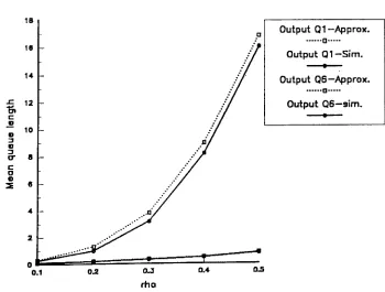
Results in figures 8 to 11 were obtained under a nonuniform destination distribution. In particular, for each
input queue 30% of the traffic was destined to output queue 1 and the remainder of the traffic was uniformly
distributed among the rest of the output queues, i.e. output queues 2 to 6 get 140/0 each. This type of traffic
pattern is referred to in the literature as the hot-spotpattern. Figures 8 to 10 give the mean queue length of
output queue 1 (hot output) and output queue 6 (a non-hot output) for the three bus service policies, TDM,
Random, and Cyclic respectively. The arrival process to each input queue was an IBP with (;2
=
50 and pincreasing from 0.1 to 0.5. Note that when p is equal to 0.5, the average rate of arrivals destined for output
I (hot output) is equal to 0.9 which is the output link capacity. For allthree bus service policies, although
not shown, the input queues were virtually empty. This is due to the fact that the bus speed is equal to the
sum of the input link capacities and as a result, most of the queueing within the switch occurs inthe output
queues. We note that there is a good agreement between the approximation results and the simulation data.
The maximum, minimum, and average relative errors for the results in figure 8 are 8.10/0, 2.60/0, and 4.9%,
and for the results in figure 8 are 14.5%
, 6.1% , and 10.6% respectively. Maximum, minimum, and average
relative errors for results in figure 8 are 14.8%, 4.90/0, and 10.70/0 respectively. Figure II gives the blocking
(PI = 0.1, P2= 0.2, P3= 0.3, P4= 0.4, ps
=
0.5, P6= 0.6, andQ= 100 for i= 1,2,...,6) and nonuniform traffic destination distribution ( the same destination distribution mentioned above). This pattern gives widevariation of traffic crossing the switch, Under TDM bus service policy, the blocking probability increases as
the input queue number is increased from I to 6 which is expected. On the other hand, under cyclic service,
the blocking probability is highest for the input queue with.the.Iowest .arrival rate and vice versa. This can
be explained, intuitively, by the fact that the heavily utilized input queues keep the hot spot output full most
of the time. Thus, blocking probabilities of the input queues with low arrival rates is increased. The
maximum, minimum, and average relative errors for the results in figure 8 are 16.70/0, 3.30/0, and 11.60/0
respectively.
In general, the accuracy of the algorithm is good. It was observed that ifthe input or output queue size is
small (i.e. less than 16) the results are not very good when C2 is high (i.e. greater than 100). When the queue
size is large (i.e. equal to or greater than 32) the accuracy is good for values of0- up to 150.
5.0
ConclusionsIn this paper, we presented an approximate analysis of a generic shared-medium ATM switch under realistic
system characteristics such as limited buffer size, asymmetric load conditions, and nonuniform destinations.
Three different bus service policies were analyzed: Time Division Multiplexing (TDM), Cyclic, and Random.
The analysis is based on the notion of decomposition whereby the switch is decomposed into smaller
sub-systems. First, each input queue is analyzed in isolation after we modify its service process. Subsequently,
the shared medium is analyzed as a separate sub-system utilizing the output process of each input queue.
Finally, each output queue is analyzed in isolation. The results from the individual sub-systems are
com-bined together through an iterative scheme. The model's accuracy is verified through simulation. It was
References
1. I. Cidon, I. Gopal, G. Grover, and M. Sidi, "Real-Time Packet Switching: A Performance Analysis",
IEEE JSAC Vol. 6 NO.9, December 1988.
2.'
A. Ganz, and I. C'Wamtac, ';A LinearSolution to Queueing Analysis of SynchronousFinit~
BufferNet-works", IEEE Trans. on Comm., Vol. 38, NO.4, April 1990.
3. S. Gershwin, "An efficient decomposition algorithm for unreliable tandem queueing systems with finite
buffers", First Int. Workshop on Queueing Networks with blocking, North Holland, 1989.
4. O. Ibe and K. Trivedi, "Stochastic Petri Net Models of Polling Systems", IEEE JSAC, Vol.8 NO.9,
December 1990.
5. F. Jou, A. Nilsson, and F. Lai, 'The Upper Bounds for Delay and Cell Loss Probability of Bursty ATM
Traffic in a Finite Capacity Polling System", Second Int. Workshop on Queueing Networks with
blocking, RTP, North Carolina, May 1992.
6. M. Karol, M. Hluchyj, and S. Morgan, "Input versus output queueing on a space-division packet
switch", IEEE Trans. Comm., VOL. 35, NO. 12, December 1987.
7. T. Morris and H. Perros, "Performance analysis of a multi-buffered Banyan ATM switch under bursty
traffic", INFOCOM 92, Florence, Italy.
8. A. Nilsson, F. Lai, H. Perrros, "An Approximate analysis of a bufferless NxN synchronous Clos ATM
switch"in: Cohen and Pack (eds.), Queueing, Performance, and Control in ATM, North-Holland, 1991,
39-46.
9. A. Pattavina, "Performance evaluation of A"fM switches with input and output queueing", International
Journal of Digital and Analog Communication Systems, VOL. 3, 1990.
10. I-I.G. Perros, HApproximation algorithms for open queueing networks with blocking", in Takagi (ed.),
11. 1-1. Suzuki, H. Nagano, T. Takeuchi, and S. Iwasaki, "Output-buffer switch architecture for
asynchro-nous transfer mode", Int. Conf. on Communications, Boston, MA, June 1989.
12. H. T~agi, "Queueing Analysis of Polling Models: An Update", in Takagi (ed.), Stochastic Analysis of
Computer and Communication Systems, North-I-IolJand, 1990,267-318.
13. F. Tobagi, "Fast Packet Switch Architectures for Broadband Integrated Services Digital Networks",
Pro-ceedings of the IEEE, Vol. 78, NO. I, January 1990.
14. P. Tran-Gia, "Analysis of Polling Systems with General Input Process and Finite Capacity", IEEE
Trans. on Cornm., VOL.40, NO.2, February 1992.
15. J.Turner, "Design of a broadcast packet switching network", IEEE Trans. Comm., Vol. 36, NO.6, June
1988.
16. A. Zaghloul and H. Perras, 1/Approximate analysis of a discrete-time polling systemwith burstyarrivals",
IFIP workshop on "Modelling and Performance Evaluation of ATM technology", Martinique, January
8p .
Bp
Bp
m
m
~
IIII1
~IIIII.I
~1111'11'~~~llrlll
.
,
I, I
.
~...
-"
~ ~III
i
111/
input links
shared mediumoutput links
Figure I. Queueing model of a shared-medium switch
Bus slots
/
.
.
~
Bus Cycle
6
~_ _ Arrival slot _ _--...--- hrivaJ slot
+
Output linA:service
completion
+
Output lint
service
completion
Pb
IBP
r--·----·-·...--··---..--...---...----·....---...---_...,
i i
I
1I . . .
i
:r
n1-Pb.
I
o -
ONE BUS SlDT TINEIr
lH~---_._---_!
Figure 3. Effective service time of an input queue (Cyclic case)
TO~-Sim.
•
Cyclic-Sim. TDM-Approx.···0···
Cyclic-Approx.···0···
..0' 1/' 3 Input queueOll.-ol.---...Io..---'""'---_ _L-..._ _--L.
....L-0.5 4-3.5 J s: 0, 2.5 c .s G ::l 2 G : ] (T c: c 1.5 G ~
Figure 4. Mean input queue length: uniform destinations, p 0.7, C2
TOM-Sim.. Cyclic-Sim.
•
TDM-Approx•···0···
Cyclic-Approx.···0···
..•.
... ... ••••••0...
.'...
& -0 -0••••••••••••••0 ••••••:.::.::.::-:.::••••
O ... -'- ..L..-.._ _-J. ...J.-_=-:>--1_ 0.04 0.035 O.OJ
~
:a
0.025 a ..0e
Q. 0.02 C' c:x
u 0.015 a (Ii 0.01 0..0052 3 4
Input queue
5 5
Figure 50 Blocking probability: uniform destinations, p 100
TDM-Sim.
•
TDM-Approx.···0···
Random-Sim. Random-Approx.···D···
...•
...
....
•••.•••.•••••••••.0. ...1J. J Input queue0 ....: ; ; ; . . . . . . " " " " ' ... '
-0.005 0.04 0.035 O.oJ
~
0.025 ..0 0 ..0e
a. 0.02 crJ"
~ 0.015 G 0 0.01Oll
0.7
0.8
s:
Otc 0.5 -..!! G ::J 0.4 0 ::J (T • c:
0 0..3
-G ::E 0.2 0.1 -0 TDM-Approx.
···0···
TDM-Sim. Random-Approx.···0···
Random-Sim.•
Figure 7. Mean queue length: asymmetric arrivals, uniform destinations
18 18 14 s: 12 0-c: .s G 10 ::J 0 :::J 0- Il
-c 0 0 ::E II 4 2 0
0.1 0.2 0.3
rho
0..4
:fJ Output Q1-Approx.
···0···
OutputC1-Sim.
Output Qa-Approx.
···0···
Output Q6-sim.
•
0.5
•
Output Q6-sim. Output Q1-Approx•···0···
Output Ql-Sim• Output Q6-Approx.···0···
0.5 0.4 0.3 rho •:0 ...6...
..si...
... 111 HI 14 .c 12 Dt c.s
D 10 :J D :J a- S c 0 G ~ tI ~ 2 0 0.1Figure 9. Mean queue length: Random selection, nonuniform destinations
•
•
output QS-sim. Output Q6-Approx.···0···
Output Q1-Approx•...
[]...
output Ql-Sim. 0.5 0.4 D..] rho •:0 •••••• ,SJ....
0.2 18 18 14 s: 12 Dt c .!! 10 G :J a :J a- S c 0 D ~ fJ 4 -2 0 0.1•
Cyclic-Sim• TDM-Approx.
···0···
TDM-Sim. Cycllc-Approx.
···0···
°llo
5 ••••••••••••••0 •...•.•..•••. 0
•••....
0.02
0.002 0.004
-~
-g
0.012.0
e
Q. 0.01 DI .
C
~ 0.008
o
OJ
0.008 0.014 0.018 0.018
0""-1.---'- ..._ _.-..100 -..10-:.