Accuracy Assessment of Interstate Highway Length
Measurement Using DEM
___________________________________________________________________________________________ William Rasdorf, Ph.D., P.E.
North Carolina State University Department of Civil Engineering
NCSU Campus Box 7908 Raleigh, NC 27695 phone: (919) 515-7637
fax: (919) 515-7908 email: [email protected]
Chris Tilley
North Carolina Department of Transportation Geographic Information System Unit
Statewide Planning Branch 1554 Mail Service Center Raleigh, NC 27699-1544 phone: (919) 715-9684
fax: (919) 212-3103 email: [email protected]
Forrest Robson, P.E.
North Carolina Department of Transportation Geographic Information System Unit
Statewide Planning Branch 1554 Mail Service Center Raleigh, NC 27699-1544 phone: (919) 250-4188 ext. 204
fax: (919) 212-3103 email: [email protected]
Hubo Cai
North Carolina State University Department of Civil Engineering
NCSU Campus Box 7908 Raleigh, NC 27695 phone: (919) 515-6454
fax: (919) 515-7908 email: [email protected]
Soren Brun, Ph.D.
North Carolina Department of Transportation Geographic Information System Unit
Statewide Planning Branch 1554 Mail Service Center Raleigh, NC 27699-1544 phone: (919) 250-4188 ext. 206
fax: (919) 212-3103 email: [email protected]
___________________________________________________________________________________________ KeyWords: accuracy assessment
ABSTRACT
Road length is part of the geometry of the roadway network. Its measurement is critical to all road inventory databases. One approach to obtaining it is to drive cars equipped with a Distance Measurement Instrument (DMI) along roads to measure mileages. This method provides accurate measurements, but it is expensive and time consuming. This paper proposes an alternative way to acquire actual road length, which is currently under consideration by the Geographic Information System (GIS) Unit of the North Carolina Department of Transportation (NCDOT). The emphasis of this study was to determine the accuracy of the proposed approach.
The proposed approach employs GIS application programs written in ARC Macro Language to calculate the actual length (surface length) along the sloped surface of highway centerlines based on elevation data and the road network geometry. This was done for all interstate highways in North Carolina. The calculated GIS results were compared with DMI measurements, which is the most accurate approach presently available to NCDOT.
Accuracy Assessment of Interstate Highway Length
Measurement Using DEM
by
William Rasdorf
Hubo Cai
Chris Tilley
Soren Brun
Forrest Robson
INTRODUCTION
This paper describes the results of a quality assessment study of highway length measurement by using the U. S. Geological Survey (USGS) National Elevation Dataset (NED) coupled with planimetric data from geographic information systems (GIS). Since errors are inherent in any type of measurement data, it is necessary to assess and quantify the combined GIS/NED data quality and decide its fitness [Beard 1999, Amrhein 1990, Karimi 2000]. In this study the issue of concern is the length of highway segments, the geometry of the state highway network.
In the methodology of this paper road lengths are calculated through surface analysis, which combines NED files and a GIS photo-edited road layer. The calculated length data are then compared to another length dataset – road lengths obtained from a distance measurement instrument (DMI). The DMI data were obtained by driving cars equipped with a DMI along roads. The DMI approach is presently the most accurate approach available to the North Carolina Department of Transportation (NCDOT). Its results serve as the base of comparison in this study. The differences between these two datasets are analyzed using statistical methods.
General Background of Study
The North Carolina Department of Transportation is updating its road inventory database [Karimi 2000]. One key item that needs to be updated is the road length measurement. Keeping exact road lengths in the road inventory database is critical because it is the foundation for maintenance of existing roads, for the development of new roads, and for transportation network analysis. It is also critical for all distance-related transportation data such as features, attributes, and events. This dataset is often stored in tables tied to linear referencing systems, all of which are based on length. The ultimate use of these length values is to enable the modeling of other attributes such as pavement characteristics or other roadway attributes [Karimi 2000, Jia 2000]. Attribute values coupled with accurate measurements and geometry provide an information resource for transportation data analysis.
However, even with the many existing technologies that are available to measure road length, the problem is not as simple as it appears to be. An efficient way to measure road length with reasonable cost and a high degree of accuracy is desired.
NCDOT has updated a portion of its road inventory using DMIs. But since DMI is expensive and time consuming, another method to obtain length measurements, using NED and GIS, is being considered.
GIS is being extensively used in the United States in the transportation industry [Vonderohe 1994, Vonderohe 1993]. The transportation community has an unprecedented opportunity over the next few years to obtain, use, and distribute spatial data by applying GIS [Fletcher 2000]. In this paper the use of GIS for obtaining highly accurate distance measurements in support of transportation analysis is explored.
Purpose of Study
Currently, road lengths are most often measured by driving a car with a quantifiably accurate DMI. An alternative method has emerged with recent developments in computer technology, measurement technology, and GIS. The actual road length can be obtained efficiently by combining elevation data with a road layer to perform a surface analysis that leads to a computer generated road length [DeMers 2000]. In order to apply this method successfully to obtain length measurements, its accuracy must be evaluated and quantified [Rasdorf 2003]. This paper seeks to determine the accuracy of this method.
NCDOT determined that for an individual road segment the level of accuracy -- an error tolerance of 0.03 mile/mile (proportional error) or 0.01 mile (absolute error) is acceptable and that for the proposed approach to be useful, 90% of the road segments must have length measurements within these error tolerances. In addition, NCDOT was also concerned that segment slope and length may have significant impact on the derived length measurements in the proposed approach. The overall purpose of this study was to decide whether the proposed GIS surface analysis computes road lengths that provide this level of accuracy and whether the accuracy is significantly influenced by the slope and/or length.
Scope and Guiding Questions
Due to the limitation of photo-edited GIS data availability, this study focused on the length measurement of all the interstate highways within North Carolina.
The guiding questions this project sought to answer were:
(1) Given NED files and GIS road layers, how can the surface length be deduced using GIS? (2) How accurate are the results of this method when compared with DMI data that are the
most accurate length measurements available to NCDOT? (3) What are the factors that significantly influence accuracy?
By answering these questions one can determine whether the proposed method is an appropriate way to obtain data for road lengths and to update transportation databases.
Significance of Study
North Carolina has approximately 78,000 miles of state-maintained roads [Karimi 2000]. For that large number of miles the use of DMI is time consuming and costly while GIS is fast and relatively inexpensive, but the quality is unknown. The significance of this study was to quantify that unknown quality. Then, an appropriate method can be chosen to obtain new roadway mileages and update the existing road inventory database.
This problem of road length measurement is not specific to NCDOT. Departments of Transportation from other states also face similar situations. Thus, the results from this study are applicable to other states and to other applications where the underlying model is a network that is amenable to GIS implementation.
When taking a broader view at this research, it provides field-verified data about data quality and accuracy issues, a major concern with GIS applications [Beard 2000, Amrhein 1990, Heuvelink 1999]. Currently, there is no systematic description of the accuracy that different technologies can achieve. With this project as a case study, one useful and in-depth view of this problem is provided.
DATA SOURCE
Four major datasets comprised of NED data, photo-edited road layer, DMI data, and a link-node database, were used in this study. Each of these is described in detail in the following subsections.
NED Data
The USGS National Elevation Dataset (NED) has been developed by merging the highest-resolution, best-quality elevation data available across the United States into a seamless raster format [USGS 2001]. NED is the result of the USGS effort to provide 1:24,000-scale Digital Elevation Model (DEM) (1"=2000'=610m) data for the conterminous US and 1:63,360-scale DEM data for Alaska [USGS 2001, USGS 2001].
NED is essentially a digital elevation model (DEM) in which terrain elevations for ground positions are sampled at either a regular or irregular horizontal intervals [Anderson 1998, USGS 2001]. The terrain (e.g. drainage basin, water supply, etc.) surface is represented by using an array with X, Y, and Z values. DEMs are readily convertible into a grid file with most commercial GIS software.
Accuracy assessment and reporting for NED is a topic being actively pursued by USGS [Osborn 2001]. The accuracy of NED varies spatially due to the variable quality of the source DEMs and therefore, NED “inherits” the accuracy of the source DEMs [Osborn 2001].
NED data involved in this study were purchased from USGS in 1998. It was developed based on 7.5-minute DEM files from USGS with most parts having 30- by 30-meter grid spacing while some parts had 10- by 10-meter grid spacing. As specified by USGS, its 7.5-minute DEMs have the vertical accuracy equal to or better than 15 meters while 90% have a vertical accuracy of 7-meter root mean square error (RMSE) or better and 10% are in the 8- to 15-meter range [USGS 2003]. Since the NED data involved in this study had taken further improvements before they were used, it is reasonable to assume that the NED data involved in this study have a vertical accuracy of 7-meter RMSE even though no formal accuracy evaluation was performed.
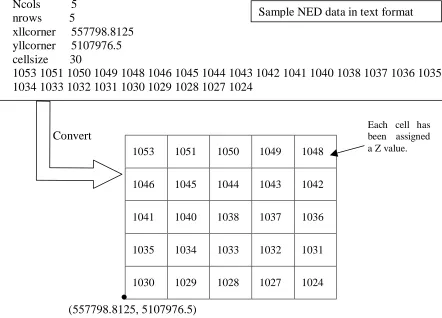
Figure 1 shows a sample NED data file in text format and illustrates how NED data are converted into a grid file (for the use of an alternative grid spacing see [Xu 2002] and [Heesom 2001].) The first two rows shown in Figure 1 specify the number of columns and rows in the file (5 rows and 5 columns for this sample file). The xllcorner and yllcorner values specify the coordinates of the start point (the leftmost, lowest point). The cell size indicates the 30 meter grid resolution. Following that is a set of numbers that specify the elevations for each cell in the sequence of rows first, top to down, and then columns, left to right. In other words, it follows the sequence of (row 1, column 1), (row 1, column 2), …, (row 1, column 5), then (row 2, column 1), (row 2, column 2), …, until it reaches (row 5, column 5).
Orthorectified Photo-edited Road Layer
North Carolina DOT maintains the roadway network in sets of Computer Aided Design (CAD) data in the format of MicroStation Design Files (DGN) for state-maintained roads, all interstate highways, U.S. Routes, NC Routes, and state-maintained secondary roads. The CAD files are readily usable in GIS through geo-referencing. The results can be stored and viewed as a thematic layer in GIS. This type of data is called road layer data in this study. This road layer data has a 1:24,000 scale. See reference [Miles 1999] for a discussion of the use of GIS in civil engineering applications.
[Heuvelink 1999, Donohoo 1990] if not corrected. In order to use this data source, it has to be revised.
The revising method used orthorectified aerial photos to correct the road layer (manually rather than automatically [Treash 2000]] by matching and digitizing the photos with the linework. The 1:24,000 target scale of the photos matched the scale of the road layer data. This revising procedure resulted in what is referred to as either the corrected or photo-edited road layer data in this paper. This photo-edited road layer includes all of the state-maintained roads mentioned above. All interstate highways were extracted from this road layer dataset for further calculations and analyses.
DMI Data
This type of data was acquired by driving cars equipped with highly precise and accurate DMI along roads to measure their lengths. A DMI is essentially an electronic receiver that works in a way similar to an odometer. It works together with sensors and an electronic amplifier. The sensors are either wheel sensors or transmission sensors depending on where they are located. When the vehicle moves, the sensors detect the vehicle movement and generate electronic pulses. These electronic pulses are preprocessed and amplified by the electronic amplifier into the suitable working rate. The pulses from the electronic interface amplifier are sent to the DMI. Based on the received pulses, the DMI counts the revolutions of the vehicle transmission (when transmission sensors are used) or the revolutions of the wheel (when the wheel sensors are used) and derives the distance the vehicle has traveled.
When properly calibrated, a DMI measures the actual length of a linear object such as a road segment at an accuracy level of ± 1 foot per mile (repeatability) or a 0.02% error as specified in the manufacturers’ specifications. In other words, when measuring a road segment with a 2-mile length, the expected error would be ± 2 feet. Presently DMI measurements are the most accurate length measurements available to NCDOT and thus they were used as the basis (reference data) for comparison and accuracy assessment in this study. DMI data are available for all interstate highways in North Carolina. They were obtained during a field measurement effort in the summer of 2000.
Link-node Database
NCDOT presently uses essentially a link-node database. This link-node database stores the length of road segments in units that can be referred to as links. These link lengths are the DMI lengths mentioned in the previous section. Details of the link-node database are not provided here because they are out of the scope of this paper. But it is this link-node database that is the source of the DMI mileage measurements that are used in the analysis described herein.
DATA ANALYSIS
show the flowcharts for these three parts respectively. The steps within each part are described in detail in the following subsections.
Surface Analysis
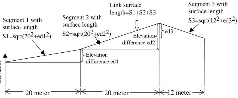
The goal of surface analysis is to calculate the actual road centerline length of the links comprising the highway network. To do so a horizontal distance obtained from the GIS linework and a vertical distance obtained from NED data are used in a GIS function to calculate a 3-dimensional true slope distance (the actual road centerline length). This can then be compared to a slope distance actually measured using DMI. Figure 2 shows the flowchart for this sequence of activities.
(1) The original NED is converted into a 30- by 30-meter grid file as was shown in Figure 1.
(2) CAD files are matched with aerial photos. If roads on the CAD files do not match roads on the orthorectified aerial photos, they are revised by digitizing the orthorectified aerial photos. The product of this step is a cleaned road layer with all roads in their correct 2D spatial positions. The cleaned road layer is then converted from a CAD file into a shapefile. By next building topology (a built-in GIS capability), the length of all links (2D planimetric length) is generated automatically by the GIS software.
(3) DMI lengths from the link-node database are provided to the road layer, along with geometry and topology information, as attributes. After this step, the so-called cleaned road layer has both 2-dimensional planimetric length (calculated by the GIS software) and 3-dimensional length (measured by DMI data) as attributes.
(4) The cleaned road layer is overlaid with the 30- by 30-meter grid file. By performing surface analysis, GIS calculates the actual 3-dimensional length for all links based on the 2-dimensional length of the cleaned road layer and the elevation information from the grid file. At this point a revised road layer with planimetric length, DMI length (measured length), and GIS generated surface length, is available for further analysis.
Suspect Links
It is recognized that all data sources have inherent errors. Some errors are from the datasets themselves, while others are introduced during the analysis procedure [Donohoo 1990, Burrough 1998, Ngan 1995]. What is being done here is to attempt removal of dataset errors so that only errors from the elevation analysis are left. These errors can then be evaluated on their own merit.
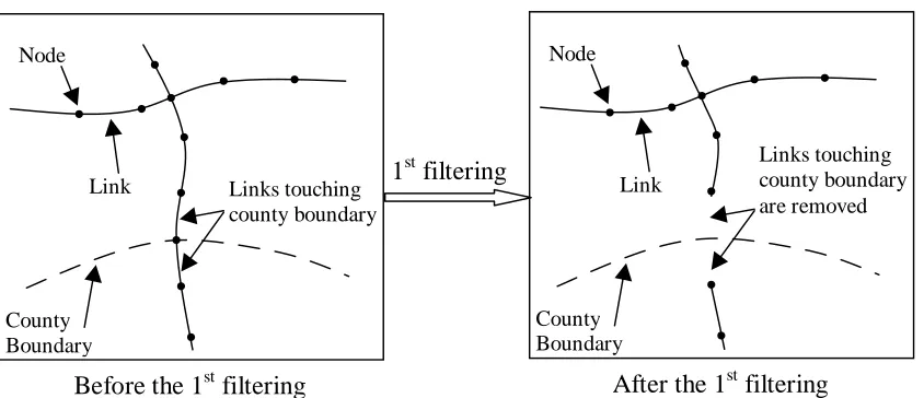
Suspect links are links that have suspect length measurements based on knowledge and experience. That is, the length stored in the database for some links is simply wrong. Three groups of suspect links were identified in this study. The first group of links that need to be removed are links that touch county boundaries. These are known to have uncertain length measurements due to the inability to exactly pinpoint the boundary during measurement because a county boundary is not a physical line, and there can be disagreement by field personnel about its precise physical location. Furthermore, a technician who is conducting a field survey may be totally unfamiliar with the roadway location. As a result, there is great uncertainty about the length of the links that border a county boundary, and subsequently, the start and end nodes for links of this group. They are not valid for accuracy assessment with any degree of certainty. They were removed from analysis by applying the 1st filter shown in Figure 4 (step 5). The concept is illustrated in Figure 5.
The second group of suspect links are those which have a 2D planimetric length that is greater than their 3D surface length (SLENGTH). This is clearly an impossible situation caused by inherent system errors in integrating raster elevation data with vector roadway data to calculate surface length. These are unavoidable inherent system errors in GIS. Because they can be identified they too are removed.
The third group of suspect links were identified by taking into consideration that most interstate links are relatively short flat links (64% of all links are less than 1 mile in length; 83% are less than 1.5 mile in length). There should be no significant difference between planimetric length and surface length. In other words, a link whose planimetric length in the database might be 0.50 mile but whose surface length is determined to be 1.00 mile is clearly suspect. There is a problem with the link itself. Most likely, the technician entering the data made a clerical error. Thus, the link would be a poor choice to use to evaluate accuracy. Any links with a planimetric/surface (DMI) length difference exceeding a tolerance level are not valid for accuracy assessment. These links were removed from accuracy assessment by applying the 2nd filter in Figure 4. Figure 6 shows how many suspect links were removed for all of the groups identified above.
Removing Suspect Links and Calculating Additional Attributes
(5) All the links touching county boundaries were individually identified and then removed by overlaying the revised road layer with the county boundary layer. Figure 5 illustrates how the 1st filter works.
(6) All the necessary attributes for future analyses, including the second filtering, grouping, and statistical analysis, were added and calculated. These new attributes include:
(a) A2DMILE, the result of converting LENGTH (computer generated planimetric length) from units of meters into units of miles;
(b) D_PMU_A2D, the difference between A2DMILE and PMUMILE (the actual length measurement from DMI);
(c) Slope and SLOPE%, the slope of links in both decimal and percent formats;
(d) DIFFERENCE, the absolute difference between PMUMILE and LENMILE (GIS length measurement);
(e) DPERMILE, which indicates the proportional difference between PMUMILE and LENMILE in units of mile/mile.
(f) SLENGHT is the slope length calculated using the SURFACELENGTH function.
(7) All the newly added attributes were calculated using on the available data. The equations used to calculate values for these attributes are as the following (in ArcView format):
A2DMILE = LENGTH/1609
DIFFERENCE = (LENMILE - PMUMILE).ABS DPERMILE = DIFFERENCE/PMUMILE D_PMU_A2D = (PMUMILE - A2DMILE).ABS SLOPE = ((SLENGTH * SLENGTH) - (LENGTH *
LENGTH)).SQRT/LENGTH
(8) The 3rd filter was applied to remove the third group of suspect links – links having absolute difference between 2D Planimetric length and 3D DMI length exceeding the tolerance. These suspect links were removed from the fully attributed road layer, which led to a final test case road layer.
One thing to observe after performing the step (7) calculation is that 66 links out of a total of 2336 links (2.8%) end up with LENGTH (2-dimensional length) longer than SLENGTH (3-dimensional length). These links are specified as the special group 2 links mentioned in the previous section. The explanation for this result is that the links within this group are relatively short links (46 links out of 66, or 70%, are less than 0.05 mile; 60 out of 66, or 91%, are less than 0.50 mile). GIS uses two different data models (raster and vector, respectively) to calculate LENGTH and SLENGTH. For short links, there is inherent system error because of scale and storage differences. Further analyses do not include these 66 deficient links.
Figure 6 shows the numbers of links removed for those three suspect link groups. This portion of the analysis has the remaining road layer as its end product. This road layer is composed of a set of links that are deemed to be valid for accuracy assessment because we have removed suspect links that were deemed invalid for analyses. The result is a reasonable dataset of links that we may now use further analysis.
Grouping and Statistical Analyses
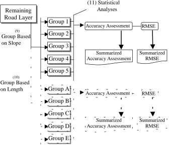
In this portion of the study, all remaining links were grouped based on slope and length. The reason for grouping based on slope and length is to determine whether slope and length are significant factors influencing accuracy of length measurement and if so, what impact they might have. After grouping, statistical analyses including frequency analysis and RMSE were conducted for all groups. The overall procedure is illustrated in Figure 7 and described by steps 9-11 below.
(9) All the links in the remaining road layer were sorted based on SLOPE, which resulted in 5 sub categorizations (Group 1 to Group 5). The slope range and number of links for each group are as follows.
Group 1 0% =< SLOPE < 2% 426 Links Group 2 2% =< SLOPE < 4% 764 Links Group 3 4% =< SLOPE < 6% 353 Links Group 4 6% =< SLOPE < 8% 96 Links Group 5 8% =< SLOPE < 24% 63 Links
All links with a SLOPE greater than or equal to 8% were included together in one group because the number of links was so small that the analysis results would otherwise have been statistically insignificant. If the Group 5 links had been divided into 2% slope ranges, there would not have been enough links within each new group to maintain the validity of statistical analysis.
(10) All links in the remaining road layer were also grouped based on PMUMILE, the measured DMI length, which resulted in another 5 categorizatinos, shown below as categorizations, A to E. The length range and number of links for each of these groups are as follows.
Group C 0.50 mile < PMUMILE <= 1.00 mile 476 Links Group D 1.00 mile < PMUMILE <= 2.00 mile 507 Links Group E 2.00 mile < PMUMILE <= 5.00 mile 119 Links
(11) Frequency analysis and RMSE were conducted for every group. Then, all the analyses and assessments were summarized together to presents the results.
ANALYSIS RESULTS
Two major categories of analyses were used to study the results. They are frequency analysis and RMSE. Frequency analysis represents the accuracy for every group by counting the number and calculating the percentage of links within certain error ranges for each group. RMSE and 95% confidence level is the other form of assessing length measurement accuracy that was used in this study.
Frequency Analysis
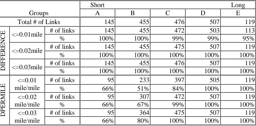
Frequency provides an in-depth way to view error distribution in percentages. Table 1 summarizes the results of frequency analysis for groups based on slope and Table 2 summarizes the results of frequency analysis for groups based on length.
Observations from frequency analysis for groups based on slope are:
(1) The performance of DIFFERENCE (absolute error) is better than DPERMILE (proportional error). The explanation for this is that most links are short links (about 35% of all remaining links are less than 0.50 mile long and 63% are less than 1 mile long). Errors are somewhat exaggerated in proportional form by dividing the absolute error by an ever decreasing length.
(2) Accuracy is good for all groups according to the criteria established by NCDOT as mentioned earlier.
• From the perspective of absolute error (DIFFERENCE), Group 5 shows the worst accuracy. However, it still has 90% of its links within a 0.01 mile error range and all of its links within a 0.02 mile error range.
• From the perspective of proportional error (DPERMILE), Group 4 and Group 5 have similar accuracy and they are worse than the other groups. But together, these 2 groups still have about 67% of their links within a 0.01 mile/mile error range and 80% of their links within a 0.03 mile/mile error range.
• Overall, 99% of all links are within the 0.01 mile absolute error tolerance and 92% of all links are within the 0.03 mile/mile proportional error tolerance.
Observations from frequency analysis for groups based on length are:
(1) The performance of DIFFERENCE is better than DPERMILE, which confirms the first observation from groups based on slope.
(2) Accuracy is good for all groups.
• From the perspective of absolute error (DIFFERENCE), Group E is the group with the worst accuracy. However, it still has 95% of its links within a 0.01 mile error range and all of its links within a 0.02 mile error range.
• From the perspective of proportional error (DPERMILE), Group A and Group B have similar accuracy and they are worse than other groups. But together, these 2 groups still have about 67% of their links within a 0.02 mile/mile error range and 77% of their links within a 0.03 mile/mile error range.
(3) Accuracy increases as the length increases. Error occurs primarily with short length groups.
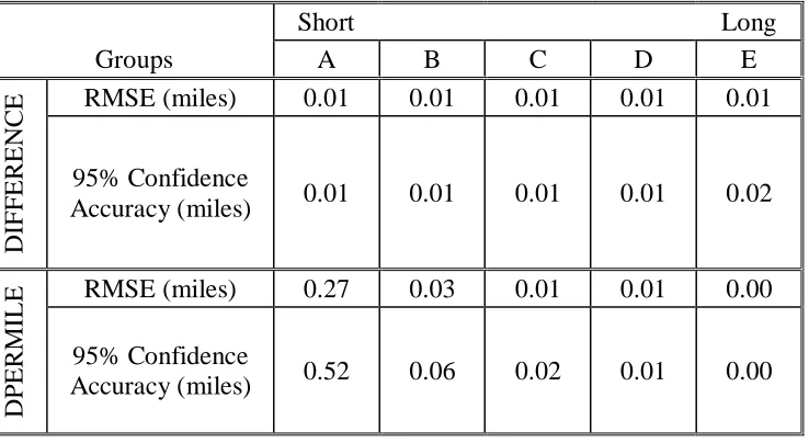
RMSE and 95% Confidence Level
RMSE is applied widely in describing differences between two datasets. In the spatial world, this statistic is often used to describe positional accuracy, including horizontal and vertical accuracy [FGDC 1998]. However, with its ability to depict the difference between two datasets, RMSE was deemed to be a useful tool for evaluating the accuracy of our results. Thus, RMSE has been calculated for all groups in this study to reveal the difference between DMI length measurements and GIS length calculations. The following equation is used to calculate RMSE [FGDC 1998].
RMSE = [(e12 + e22 + e32 + … + en2)/n] ½; e1, e2, e3, …, en ---- errors
From these two tables, similar observations may be deduced as were previously deduced by frequency analysis.
(1) The performance of DIFFERENCE is better than DPERMILE.
(2) Accuracy is good.
• From the perspective of absolute error (DIFFERENCE), links of Group 1, 2, and 3 have 95% probability of having errors no larger than 0.005 mile as indicated by the 95% confidence level, 0.00 mile. Links from Group 4 and 5 have 95% probability of having less than 0.02 mile absolute error. Groups based on length indicate that a link from groups A, B, C, or D has a 95% probability of having less than 0.01 mile error while a link from group E has a 95% probability of having less than 0.02 mile error.
• From the perspective of proportional error (DPERMILE), links from group 1 have 95% probability of having less than 0.04 mile/mile proportional error. Links from groups 2, 3, and 4 have 95% probability of having less than approximately 0.17 mile/mile proportional error. Groups B, C, D, and E have the 95% confidence accuracy of 0.06 mile/mile, 0.02 mile/mile, 0.01 mile/mile, and 0.00 mile/mile respectively. Groups A and 5 have the worst results (about 0.50 mile/mile), which correspond to the group with the shortest links and the group with the highest slopes respectively. However, because there were so few of them it is not certain that this is in reality the case. The group size is not large enough to give statistically significant results.
SUMMARY AND CONCLUSIONS
Accurate mileages are critical for the effective operations of state DOTs. This study identifies a path for these DOTs to take to acquire accurate mileages in a faster and less costly way than ever before. These mileages are the slope distance along the path of the roadway. Clearly, one way to obtain these mileages is through the use of DMI. However in those cases (and for States) where this is not practical, an alternative approach is emerging using DEMs.
This study revealed that the proposed method of using GIS + NED to calculate center line surface lengths for interstate highway links provides accurate results for this application. Thus, the method can be readily used to calculate road lengths for transportation databases with the currently available DEMs. This proposed method would have the dual implact of improving the quality of transportation databases and also of saving money and time for state DOTs.
The results of this study show that when you have accurate planimetric distances, elevations calculated from DEM data will give a degree of slope distance accuracy that is acceptable to most DOT applications. This implies that current DEM data and straightforward algorithms to calculate accurate road mileages can be immediately used to determine mileages.
Furthermore, it should be noted that geographers are continually conducting research to improve the accuracy of elevation models. Instrumentation is evolving that adds improved measurement accuracy. Thus, given that existing DEM data gives good results, the future looks even better.
Getting consistent base line data for GIS/DEM is important [Karimi 2000]. Still, it is somewhat fixed in time. No state is going to repeatedly photo-revise all of its roads, as this is not practical. Thus, once roads are photo-revised, the planimetric distances are unlikely to be changed very often. More accurate elevations, on the other hand, can be obtained whenever available, and new mileages can be calculated quickly using algorithms. Accuracy of mileages can only get better as technology improves.
What does all of this tell us? That:
• CAD or GIS road layers must consist of accurate, photo-revised, and edited lines. • DEM data can be used to calculate roadway mileages rather than having to use DMI to
physically measure them.
• Even greater improvements in elevation accuracy are on the way and this will improve our future applications' accuracy.
REFERENCES
Beard 2000 Beard, M. K. and Buttenfield, B. P. (1999). Geographic Information Systems – Principles and Technical Issues – Volume 1 – Detecting and Evaluating Errors by Geographical Methods, John Wiley & Sons, New York, Chapter 15, pages 219-233.
Amrhein 1990 Amrhein, C. G. and Schut, P. (1990). “Data Quality Standards and Geographic Information Systems,” Proceedings of National Conference ‘GIS for the 1990’s,’ Canadian Institute of Surveying and Mapping, pages 918-930, March 5-8.
Vonderohe 1994Vonderohe, A. P., Travis, L., Smith, R. L., and Tsai, V. (1994). “Adapting Geographic Information Systems for Transportation,” Transportation Research News, No. 171, Transportation Research Board, March.
Vonderohe 1993Vonderohe, A. P., Travis, L., Smith, R. L., and Tsai, V. (1993). “Adaption of Geographic Information Systems for Transportation,” NCHRP Technical Report 359, Transportation Research Board.
Fletcher 2000 Fletcher, D. R. (2000). “Geographic Information Systems for Transportation: A Look Forward,” Transportation in the New Millennium, Transportation Research Board.
DeMers 2000 DeMers, M. N. (2000). Fundamentals of Geographic Information Systems, 2nd Edition, John Wiley & Sons, New York, Chapters 8, 10, pages 208-234, 256-297.
Rasdorf 2003 Rasdorf, W., Cai, H., Tilley, C., Brun, E., Karimi, H., and Robson, F. (2003), "Transportation Distance Measurement Data Quality," Journal of Computing in Civil Engineering, American Society of Civil Engineers, Volume 17, Number 2 Pages 1-13, April.
Heuvelink 1999. Heuvelink, G. B. M. (1999). Geographic Information Systems – Principles and Technical Issues - Vol. 1 – Propagation of Error in Spatial Modeling with GIS, John Wiley & Sons, New York, Chapter 14, pages 207-217.
USGS 2001 USGS National Elevation Dataset. (2001). May 9, 2001. http://gisdata.usgs.net/ned/. Accessed May 26.
USGS 2001 USGS National Elevation Dataset. (2001). May 9, 2001. http://gisdata.usgs.net/ned/About.htm. Accessed May 26.
USGS 2000 National Elevation Dataset. (2001). USGS Mapping Applications Center,
http://mac.usgs.gov/mac/isb/pubs/factsheets/fs14899.html. Accessed October 15.
Anderson 1998 Anderson, J. M. and Mikhail E. M. (1998). Surveying Theory and Practice, 7th Edition, WCB/McGraw-Hill, Chapter 13, pages 742-779.
USGS 2001 USGS, Western Geographic Science Center. (2001). Digital Elevation Model, March 28, 2001. http://craterlake.wr.usgs.gov/dem.shtml. Accessed June 2.
Donohoo 1990 Donohoo, M. S. (1990). “Cartographic Quality Control: No Longer Optional for Today’s GIS Programs,” Proceedings of AM/FM Conference ΧΙΙΙ, pages 78-87, April.
Burrough 1998 Burrough, P. A. and McDonnell, R. A. (1998). Principles of Geographic Information Systems – Errors and Quality Control, Oxford University Press, Chapter 9, pages 220-240.
Ngan 1995 Ngan, S. (1995). “Digital Quality Control for Manual Digitizing Operations,” Proceedings of Ninth Annual Symposium on Geographic Information Systems, Vancouver, British Columbia, Canada, page 739, March 27-30.
FGDC 1998 FGDC. (1998). “Geospatial Positioning Accuracy Standards,” Subcommittee for Base Cartographic Data, Federal Geographic Data Committee, 2001. FGDC-STD-007.3-1998, http://www.fgdc.gov/standards/status/sub1_3.html. Accessed June 16.
Jenness 2001 Jenness, J. (2001). “Surface Tools for Points, Lines, and Polygons,” (v.1.2),
June 5, 2001.
Http://gis.esri.com/arcscripts/details.cfm?CFGRIDKEY=C4F41249-4FD9-11D5-944200508B0CB419. Accessed June 5.
Osborn 2001 Osborn, K., List, J., Gesch, D., Crowe, J., Merrill, G., Constance, E., Mauck, J., Lund, C., Caruso, V., and Kosovich, J. (2001), “National Digital Elevation Program (NDEP),” Digital Elevation Model Technologies and Applications: The DEM Users Manual, Editor Maune, F. D., American Society for Photogrammetry and Remote Sensing, Bethesda, Maryland 20814, pages 83-120.
USGS 2003 “USGS Digital Elevation Data Model,”
http://edcwww.cr.usgs.gov/glis/hyper/guide/usgs_dem, Accessed March 2003.
Heesom 2001 Heesom, D. and Mahdjoubi, L. (2001). "Effect of Grid Resolution and Terrain Characteristics On Data From DTM," Journal of Computing in Civil Engineering, Vol. 15, No. 2, pages 137-143, April.
Parsons 2000 Parsons, R. L., and Frost, J. D. (2000). "Interactive Analysis of Spatial Subsurface Data Using GIS-Based Tool," Journal of Computing in Civil Engineering, Vol. 14, No. 4, pages 215-222, October.
Achorya 1997 Achorya, B. and Chaturvedi, A. (1997). "Digital Terrain Model: Evaluation, Extraction, and Accuracy Assessment." Journal of Surveying in Engineering, American Society of Civil Engineers, Vol. 132, No. 2, Pages 71-76.
Karimi 2000 Karimi, H. A., Khattak, A. J., and Hummer, J. E. (2000). "Evaluation of Mobile Mapping Systems for Roadway Data Collection," Journal of Computing in Civil Engineering, Vol. 14, No. 3, pages 168-173, July.
Jia 2000 Jia, X. (2000). "IntelliGIS: Tool For Representing and Reasoning About Spatial Knowledge," Journal of Computing in Civil Engineering, Vol. 14, No. 1, pages 51-59, January.
Treash 2000 Treash, K., and Amaratunga, K. (2000). "Automatic Road Detection in Grayscale Aerial Images," Journal of Computing in Civil Engineering, Vol. 14, No. 1, pages 60-69, January.
FIGURES
FIGURE 1 Conversion of NED data into an NED grid file. FIGURE 2 Transformation from data analysis to surface analysis.
FIGURE 3 Calculations of surface lengths using ESRI SURFACELENGTH function FIGURE 4 Data analysis link filtering and additional attribute calculation.
FIGURE 5 Conceptual visualization of 1st filtering. FIGURE 6 Removing suspect links from further analyses. FIGURE 7 Data analysis grouping and statistical analyses.
TABLES
TABLE 1 Frequency Analysis for Groups Based on Slope TABLE 2 Frequency Analysis for Groups Based on Length
Ncols 5 nrows 5
xllcorner 557798.8125 yllcorner 5107976.5 cellsize 30
1053 1051 1050 1049 1048 1046 1045 1044 1043 1042 1041 1040 1038 1037 1036 1035 1034 1033 1032 1031 1030 1029 1028 1027 1024
1053 1051 1050 1049 1048
1046 1045 1044 1043 1042
1041 1040 1038 1037 1036
1035 1034 1033 1032 1031
1030 1029 1028 1027 1024
FIGURE 1 Conversion of NED data into an NED grid file.
Each cell has been assigned a Z value. Convert
Sample NED data in text format
FIGURE 2 Transformation from data analysis to surface analysis.
FIGURE 3 Calculations of surface lengths using ESRI SURFACELENGTH function
NED Convert(1) 30- by 30-meter
Grid File
CAD Files
Aerial Photos
Cleaned Road Layer (2) Match and Digitize
Link-node Database
(3) Provide DMI length
2D planimetric length 3D actual length from DMI
Revised Road Layer (4) Surface
Analysis
2D planimetric length 3D actual length from DMI 3D actual length from GIS surface analysis
20 meter 20 meter 12 meter
Segment 1 with surface length S1=sqrt(202+ed12)
Segment 2 with surface length
S2=sqrt(202+ed22)
Segment 3 with surface length
S3=sqrt(122+ed32)
Elevation difference ed1
Elevation difference ed2
ed3
E
le
v
at
io
n
FIGURE 4 Data analysis link filtering and additional attribute calculation.
FIGURE 5 Conceptual visualization of 1st filtering.
Revised Road Layer
County Boundary
(5) the 1st Filtering
Filtered Road Layer
(6) Add attributes
(7) Calculate attributes*
Fully Attributed Road Layer A2DMILE SLOPE, SLOPE% DIFFERENC E
DPERMIL E
D_PMU_A2D
Remaining Road Layer (8)
the 3rd Filtering
Road layer without links having suspect length values
County Boundary
Node
Link Links touching county boundary
County Boundary
Node
Link
Links touching county boundary are removed 1st filtering
Before the 1st filtering After the 1st filtering
(1) These 185 links touch county boundaries;
(2) These 66 links have 2D planimetric length greater than 3D DMI length;
(3) These 383 links have a difference between 2D length and 3D length exceeding a tolerance.
FIGURE 6 Removing suspect links from further analyses.
FIGURE 7 Data analysis grouping and statistical analyses.
TABLE 1 Frequency Analysis for Groups Based on Slope
Flat Steep
Groups Group 1 Group 2 Group 3 Group 4 Group 5 All
Total # of Links 426 764 353 96 63 1702
<=0.01 # of links 426 762 351 92 57 1688
mile % 100% 100% 99% 96% 90% 99%
<=0.02 # of links 426 764 353 96 62 1701
mile % 100% 100% 100% 100% 98% 100%
<=0.03 # of links 426 764 353 96 63 1702
D IF F E R E N C E
mile % 100% 100% 100% 100% 100% 100%
<=0.01 # of links 372 602 268 62 45 1349
mile/mile % 87% 79% 76% 65% 71% 79%
<=0.02 # of links 398 677 302 75 48 1500
mile/mile % 93% 89% 86% 78% 76% 88%
<=0.03 # of links 409 704 320 75 52 1560
D P E R M IL E
mile/mile % 96% 92% 91% 78% 83% 92%
TABLE 2 Frequency Analysis for Groups Based on Length
Short Long
Groups A B C D E
Total # of Links 145 455 476 507 119
# of links 145 455 472 503 113
<=0.01mile
% 100% 100% 99% 99% 95%
# of links 145 455 475 507 119
<=0.02mile
% 100% 100% 100% 100% 100%
# of links 145 455 476 507 119
D IF F E R E N C E <=0.03mile
% 100% 100% 100% 100% 100%
# of links 95 233 397 505 119
<=0.01
mile/mile % 66% 51% 84% 100% 100%
# of links 95 307 472 507 119
<=0.02
mile/mile % 66% 67% 99% 100% 100%
# of links 95 364 475 507 119
D P E R M IL E <=0.03
TABLE 3 RMSE and 95% Confidence Accuracy for Groups Based on Slope
Flat Steep
Groups GP1 GP2 GP3 GP4 GP5
RMSE (miles) 0.00 0.00 0.00 0.01 0.01
D
IF
F
E
R
E
N
C
E
95% Confidence
Accuracy (miles) 0.00 0.00 0.00 0.02 0.02
RMSE (miles) 0.02 0.06 0.08 0.12 0.25
D
P
E
R
M
IL
E
95% Confidence
Accuracy (miles) 0.04 0.12 0.17 0.23 0.49
TABLE 4 RMSE and 95% Confidence Accuracy for Groups Based on Length
Short Long
Groups A B C D E
RMSE (miles) 0.01 0.01 0.01 0.01 0.01
D
IF
F
E
R
E
N
C
E
95% Confidence
Accuracy (miles) 0.01 0.01 0.01 0.01 0.02
RMSE (miles) 0.27 0.03 0.01 0.01 0.00
D
P
E
R
M
IL
E
95% Confidence