Adaptive behavior and interference in the functional response of predator to prey

Abstract

Skalski, Garrick Tyson. Adaptive behavior and interference in the functional response of predator to prey. (Under the direction of James F. Gilliam and Nick M. Haddad)

The behavior of individuals in predator-prey interactions plays a fundamental role in population ecology and evolution. Accordingly, the development and assessment of theory that provides a conceptual framework for understanding and predicting behavior in predator-prey systems is of basic importance. This dissertation is focused on

developing and assessing theory that provides a quantitative structure for predator-prey interactions.

Chapter 1 provides a theoretical treatment of the problem of modeling the behavior of an animal facing two- and three-way tradeoffs among growth, mortality and reproduction, three components of Darwinian fitness. In this situation benefits in terms of one fitness component can be obtained only with a cost in terms of another fitness

component. Applying a dynamic optimization method, the theory describes the behavior of phenotypes that adaptively balance growth, mortality and reproduction in a size-structured population. One simple prediction of the theory is that non-growing adults in a stable population should behave so as to minimize the ratio of mortality rate to birth rate. A further extension of the theory using the idea of ideal-free distributions results in a prediction of a positive and linear relationship among the rates of growth, mortality and birth when measured across different habitat patches. These and other results lead to testable predictions and I discuss empirical examples of how subsets of the theory have been and can be assessed.

19 data sets from the literature. The results show that predator-dependent functional responses (i.e., forms that are functions of predator and prey abundance because of predator interference) provide better descriptions of 18 of the 19 data sets than the Holling Type II model, a commonly used prey-dependent functional response (i.e., a model that depends only on prey abundance). Hence some form of predator interference is common in these data. However, no single functional response can best describe all of the data sets. A key result is that the best-fitting predator-dependent model depends on the presence or absence of predator-dependence when prey are very abundant.

Accordingly, I suggest use of the Beddington-DeAngelis or Hassell-Varley model when predator feeding rate becomes independent of predator density at high prey density, and use of the Crowley-Martin model when predator feeding rate is decreased by higher predator density even when prey density is high. These results suggest that predator-dependent functional responses should be more widely considered in the literature.

predator-maintained mortality hazard. A comparison of the two best-fitting models leads to the inference that reproductive value in the bluehead chub should be thought of as a function of body size and age rather than a function of body size alone. A key implication of this result is that risk-taking behavior in these fish can be quantitatively estimated using a parameter that incorporates the benefits of growth and the costs mortality into a single fitness-based metric. The metric, called the marginal rate of substitution of mortality rate for growth rate, provides a link between behavior and life history in the bluehead chub.

Dedication

Personal Biography

I was born Garrick Tyson Skalski on March 20, 1973 in Detroit, M. I., U. S. A. Growing up in downtown Detroit, I acquired a respect for experiences that only urban living can generate: walking 100 yards to elementary school, walking 2000 yards to buy cheese, meat, and fresh produce from the farmer’s market, the Detroit Tigers winning the 1984 World Series, skate boarding to Greektown to play in the arcade perpetually

occupied with middle-aged Greek men dealing cards, football and baseball with pals in an undeveloped city lot, being white and male and in the minority in a community of folks with diverse ethnic histories, walking downtown to ice skate in the amphitheatre along the Detroit River, neighborhood unity tested by an occasional burglary or purse-snatching, having friends that also like teams from the Bad Boys era of the Detroit

Pistons, playing street hockey at the farmer’s market during a day off from school, dining out for Soul Food, and, finally, making fun of people that live in the suburbs.

Just before beginning the eighth grade my family and I moved to Asheville, N. C., U. S. A. Moving from a very urban setting to a very rural setting required a large

college at the University of North Carolina at Chapel Hill and settled on a major in Biology. After taking Biology 54, Ecology and Population Biology, I realized that this is the field where I can find out about what’s happening in those creeks. I was fortunate to have the opportunity to conduct research on the ecology of stream invertebrates under Professor Seth. R. Reice. During this experience I read and wrote about the ecological literature and participated in discussion sessions with Dr. Reice, his graduate students, and other undergraduates in the Reice Lab. It was in this setting that I was encouraged to develop a taste for theoretical approaches to biology, especially ecology.

I realized that all aspects of college life at UNC should not be taken for granted, be they scholarly or otherwise. As such, I participated fully in the aesthetic and social experiences that can only be offered by Chapel Hill: the student section on a Saturday at Kenan Stadium, meeting friends for beer at He’s Not Here on a warm afternoon, riding my bike (bike as in motorcycle) around town and through the countryside of Orange County, pulling for the Tarheels come tournament time in the TV lounge of Stacy dormitory, talking with friends the next morning about all of the stupid events of last night, picking up a keg from TJ’s, living at the residences of Barclay and Ashley Forest, playing hoops after class on the outdoor court near Cobb Hall, eating at Time Out, and going for a leisurely, mainly pointless, stroll through campus on a clear blue day with roommates.

Acknowledgments

I am thankful for the assistance of many individuals during the course of my graduate training. The staffs of the Departments of Zoology and Statistics kept the paperwork flowing and the computers running. I am appreciative of the many fun and intelligent fellow graduate students that I have gotten to know over the years - I’m glad that we never take ourselves too seriously. I benefited from many excellent classroom teachers on the faculty at N. C. State, especially Roger Berger, John Bishir, Ernest Burniston, David Dickey, Steve Ellner, Tim Elston, John Franke, Joe Hightower,

Table of Contents

Preface ix

List of Tables xii

List of Figures xiii

Chapter 1: Adaptive behavior in a size-structured population: three way tradeoffs

among growth, mortality and reproduction…………..……… 1

Abstract………. 2

Introduction………... 3

Adaptive Behavior in a Size Structured Population……….. 5

Testing Optimization Models of Behavior……… 14

Conclusions………... 22

Literature Cited……….. 24

Figure Legends………... 28

Chapter 2: Functional responses with predator interference: viable alternatives to the Holling Type II model …………..……… 31

Abstract………. 32

Introduction………... 33

Methods……….……… 39

Results………..………. 43

Discussion………..……... 46

Acknowledgments………. 51

Literature Cited……….. 52

Figure Legends……….. 62

Appendix 1……… 65

Appendix 2……… 68

Chapter 3: Feeding under predation hazard: testing models of adaptive behavior with stream fish………... 73

Abstract………. 74

Introduction………... 75

Methods……….……… 77

Experimental System………. 77

Growth Experiment……….. 77

Behavioral Experiments……… 79

Experiment One…...………. 81

Experiment Two…..………. 82

Alternative Optimization Models of Behavior………. 83

Statistical Model Selection………..………. 90

Growth Experiment……….. 93

Behavioral Experiments……… 94

Discussion………..……... 98

Acknowledgments………. 106

Literature Cited……….. 107

Preface

The content and philosophy of this dissertation reflect the content and philosophy of the training that I have received and pursued as a graduate student. I have attempted to apply the best concepts from my schooling to the problem of scientific discovery. Five themes form the philosophical basis for this work.

First, I believe that research in biology should be firmly rooted in natural history. Biological pattern and process, if we interpret it correctly, should fall directly within the context of evolution in the field. I have attempted to make my studies, no matter how abstract, based on observations and information from organisms in the wild. In my theoretical work this means tracking relevant state variables and generating predictions that can be measured. In my empirical work this means taking measurements that can be, at least by analogy, extrapolated to field settings.

“God does not care about our mathematical difficulties. He integrates empirically.” - Albert Einstein

Second, in the context of ecology and evolutionary research, I feel that the

behavior of animals plays a vital, fundamental role. If we are interested in the population-level phenomena that form the core of ecological and evolutionary thought, then a

“The difficulty in most scientific work lies in framing the questions rather than in finding the answers.” - A. E. Boycott

Third, I believe that biological investigation is strengthened by the application of mathematical tools. Mathematical models make theory less ambiguous and statistics permits a determination of empirical uncertainty. As the science of biology progresses quantitative approaches will become increasingly relevant and prevalent in the discipline. Hence my dissertation draws heavily on some basic tools of applied mathematics.

“Every new body of discovery is mathematical in form, because there is no other guidance we can have.” - Charles Darwin

Fourth, I am an advocate of simultaneously utilizing empirical and theoretical approaches. It is clear that science can not progress on the strength of theory or

empiricism alone. As such, it is reasonable to conclude that the integration of theory and data provides more information about the object(s) of inquiry than either approach used alone. My dissertation corroborates this notion: the models and data from Chapters 2 and 3 are hardly novel in isolation and only the assessment of the models using the data makes a substantial scientific contribution.

and digested. Therefore, from a closer and purer league between these two faculties, the experimental and the rational (such as has never been made), much may be hoped.” -Francis Bacon

Fifth, and finally, I adopt the philosophy that science is best advanced by considering the relative merits of alternative hypotheses. It’s clear, in biology at least, that the available scientific hypotheses are approximations and incomplete descriptions of nature, at best. Thus, a reasonable approach is to hope to improve these approximations iteratively via application of the scientific method. Accordingly, in the analysis of data in my dissertation I embrace this approach and consider several alternative hypotheses.

“The young specialist in English Lit, ...lectured me severely on the fact that in every century people have thought they understood the Universe at last, and in every century they were proved to be wrong. It follows that the one thing we can say about our modern ‘knowledge’ is that it is wrong.

List of Tables

Chapter 2

Table 1: Functional Responses in the Ecological Literature……….… 59 Table 2: Functional Response Data Sets………... 60

Chapter 3

List of Figures

Chapter 1

Figure 1: Two Hypothetical Behavioral Options Sets……...………29 Figure 2: Graphical Solutions for Optimal Behavior……….30

Chapter 2

Figure 1: Comparative Fits of Functional Response Models……… 63 Figure 2: Representative Fits of Predator-Dependent Forms……… 64

Chapter 3

Figure 1: Graphical Solutions of Optimal Behavior……….. 117 Figure 2: Fit of the Growth Model to the Data……….. 118 Figure 3: Fit of Model 1 (maximize growth) to the Data……….. 119 Figure 4: Fit of Model 2 (minimize mortality) to the Data……….………...120 Figure 5: Fit of Model 3 (minimize mortality/growth) to the Data………... 121

Chapter 1

Abstract

Predicting behavioral phenotypes is an important goal in ecology and evolution, but the task is made challenging by the fact that Darwinian fitness is comprised of several components that can not usually be simultaneously optimized (i.e., increases in one component are achieved only with the cost of decreasing other components). Here I explore a theoretical representation of the problem of an animal balancing two- and three-way tradeoffs among growth, mortality and reproduction in a size-structured population, review approaches used for testing some of the theory and consider two empirical examples from the literature. The formulation is a direct extension of earlier work and provides expressions that predict adaptive behavior in the presence of two- and three-way tradeoffs. One parsimonious result is that non-growing adults in a stable population should behave so as to minimize the ratio of mortality rate to birth rate. A further

Introduction

Modern evolutionary biology rests upon the Darwinian theory that animals evolve so as to maximize fitness subject to certain constraints. Ecologists have applied ideas involving fitness maximization to a variety of ecological problems, especially the

problems of predicting behavioral (e.g., MacArthur and Pianka 1966, Fretwell and Lucas 1970, Charnov 1976) and life history phenotypes (e.g., Williams 1966, Gadgil and Bossert 1970, Schaffer 1974, Taylor et al. 1974, Perrin and Sibly 1993) that could result from natural selection. Many mathematical representations of fitness are difficult to measure in nature and many of the attempts to predict behavior based on fitness

considerations utilize a single component of fitness, such as feeding rate (e.g., Milinski 1979, Harper 1982), mortality rate (e.g., Godin and Dugatkin 1996), or birth rate (e.g., Parker 1978), as a proxy for fitness (Stephens and Krebs 1986, Krebs and Davies 1993, Houston and McNamara 1999). Other studies emphasize the idea that different

components of fitness, such as feeding rate, mortality rate, and birth rate, contribute, perhaps in conflict, to determine an organism’s fitness (e.g., Milinski and Heller 1978, Sih 1980, Werner et al. 1983, Mangel and Clark 1988, Houston and McNamara 1999). For example, a behavior that yields the highest feeding rate may also yield the highest mortality rate. In fact, a large literature now exists to support the statement that animals consider different components of fitness when making behavioral decisions (Lima and Dill 1990, Milinski 1993, Lima 1998). Moreover, a theoretical framework for

While the empirical literature has shown that animals are likely to consider different components of fitness, data that assess how animals may quantitatively balance the conflicting demands of these components in terms of fitness consequences are lacking. Specifically, the available empirical analyses address the presence or absence of a role for potential fitness components, but do not explore how these components tradeoff using the framework of available theory. An empirical difficulty imposed by many theories is the need for estimates of marginal rates of substitution. These rates allow for the differing components of fitness to be assessed in terms of the common currency of reproductive value (Brown 1992, Houston and McNamara 1999). However, the marginal rates of substitution, as one might surmise, involve reproductive value, a quantity that is difficult to measure directly.

In an effort to facilitate empirical efforts, Gilliam (1982) introduced a

simplification to the theory that partially negated the need to estimate marginal rates of substitution and quantities involving reproductive value in order to predict behavior (see also Werner and Gilliam 1984). Yet despite this simplification, Gilliam’s most useful result, that some animals may behave so as to minimize the ratio of mortality rate to growth rate, has hardly been assessed (Lima and Dill 1990, Lima 1998). Accordingly, in this chapter my intent is stimulate empirical research along these lines: research that rigorously tests hypotheses concerning two-way and three-way behavioral tradeoffs involving rates of growth, mortality and reproduction.

I develop and analyze a generalization of the basic size-structured model

rates of growth, mortality and reproduction. I then discuss the most relevant set of empirical literature and approaches for testing the theory.

Adaptive behavior in a size-structured population

I propose a simple extension of Gilliam’s (1982) size-structured model (see also Werner and Gilliam 1984). Except in one aspect, my model is essentially identical to Gilliam’s (1982) earlier model. Like Gilliam (1982), I assume that the individuals in the model population can be categorized by a single state variable, s, which could be any biologically relevant feature of the organism’s state, including, for example, age, body size, level of energy reserves, or territory size. For illustrative purposes I take the state variable to be body size. I assume that an individual’s reproductive value, V, is given by a function of one variable, the state variable, giving V=V(s). Hence reproductive value is independent of age and time of year with the implications that there exists no maximum age and all constraints are independent of age and time of year (e.g., no seasonality in mortality or reproduction).

My extension is to assume that individuals face behaviorally-mediated tradeoffs

among rates of growth, g, (i.e., changes in the state variable), mortality, µ, and birth, b, giving a three-way tradeoff (in contrast, Gilliam (1982) considers the growth-mortality tradeoff only, a two-way tradeoff, and takes b as a given function of s). I model these

tradeoffs by writing µ=µ(s, g, b) with the constraint equation h(s, g, b)≤0. The functions

µ(s, g, b) and h(s, g, b) are given: they are taken to be completely determined by the

details of the population (e.g., the habitat and density of the population) and its

the model through g and b. One can think of an organism as having a set of behavioral options, each resulting in a growth rate, g, and a birth rate, b, which then, along with the

organism’s state, s, determine the mortality rate via the function, µ. The equation h(s, g,

b)≤0 can be thought of as a size-specific constraint on the set of biologically possible values for g and b (e.g., an animal can not allocate 100% of its time to feeding and 100% of its time to nest building). Thus each behavioral option can be specified by a vector (g,

b, µ) which is sufficient to completely specify the fitness consequences of each behavior at each body size. Throughout my analysis I consider the functions µ and h to be

increasing in g and b because I am studying tradeoffs among fitness components.

One can interpret mortality rate as a function of g and b in a variety of ways. For example, a set of behavioral options for an animal may be a finite number of choices of

different habitats, with each habitat described by a point (g, b, µ). In this case, the set of behavioral options is a finite number of points (Fig. 1a). For an animal that spends some proportion of its time in more than one habitat then the set may be extended to include all linear combinations of the available habitats resulting in a 3-dimensional polygon (Fig. 1a). In contrast, the set of behavioral options may be determined, for example, by the proportions of time that an animal spends feeding and building its nest. In this case the set of behavioral options may be a 3-dimensional region with a smooth surface if the

vector (g, b, µ) is a smooth function of the proportion of time allocated to each activity

(Fig. 1b). For the purposes of my analysis, I define the behavioral phenotype as the set of

behavioral options employed by an organism over its lifetime (i.e., the choice of (g, b, µ) employed at each body size). My analytical approach is to identify and study the

My analysis only considers the properties of phenotypes, and does not explicitly consider the genetics that may underlie these phenotypes. Hence my approach should be interpreted as identifying optimal behavioral phenotypes that can serve as evolutionary stable strategies, without consideration of the more complicated and general problem of describing dynamical evolution (Leon 1976, Charlesworth 1980, Houston and McNamara 1999, Kozlowski 1999). Although my model may indeed approximate the evolutionary dynamics of some particular genetic systems (Leon 1976, Charlesworth 1980), in general my results are best interpreted as representing potential phenotypic endpoints of

evolution - with no explicit specification of how such endpoints may be reached by evolving populations (Houston and McNamara 1999).

Using reproductive value as the metric of fitness, I study the optimal behavioral phenotype of individuals within a small sub-population that is invading a larger base population (Leon 1976, Kozlowski 1999). By definition, reproductive value for a growing organism, when parameterized by body size (by employing the change of variables ds/g=dx in the standard integral equation for reproductive value with age=x) is given by ) ( ) ( ) ( ) ( ) ( 0 ) ( s s l dw w g w b s w l e s V s w R

∫

∫

∫

and s0 is the body size of a newborn (Werner and Gilliam 1984). The growth and birth

rates are written as functions of body size, g=g(w) and b=b(w), because behavioral decisions, and hence g and b, are expected to vary with body size. Thus, my goal is to identify the functions g(s) and b(s) such that fitness is maximized.

Parameterized by only the state variable, s, it suffices to track changes in

reproductive value as body size changes. In a growing organism, reproductive value, for small changes in body size, ∆s, satisfies the recursive relationship

) ( ] 1 [ )

( sV s s

g r s g b s

V = ∆ + − +µ∆ +∆ .

Taking the limit as ∆s becomes small and applying the result that optimal behavioral phenotypes maximize reproductive value at every body size through the appropriate choices of g and b (e.g., Schaffer 1974, 1983, Taylor et al. 1974), gives the dynamic programming equation     ₋ + =

− * max *

, V g r g b ds dV b g µ

subject to h(s,g,b)≤0, (1)

have assumed a priori. Accordingly, the functions µ and h along with the dynamic

programming equation completely specify the problem of finding optimal choices for g(s) and b(s).

The computation of the optimal population growth rate of the invading sub-population, r*, is a two-step process (Leon 1976, Gilliam 1982, Taylor et al. 1974). First one finds the optimal behavioral phenotype (i.e., the optimal functions g*(s) and b*(s)) treating r (the growth rate of the base population) as a given parameter. In general, the functions g*(s) and b*(s) will also be functions of r. In the second step the functions g*(s) and b*(s) are substituted into the Euler-Lotka equation (i.e., the equation V(s0)=1)

which is then solved to obtain the optimal growth rate of the invading sub-population, r* (r* is thus a function of r). The actual computation of r* is not necessary for this analysis, as I will not specify particular forms for the functions µ and h. Keeping these ideas in

mind, in the following sections I treat r as a given parameter with r V

b

≤

−µ at every size

(otherwise the animal does not grow or reproduce).

The fundamental results of this analysis are given by carrying out the maximization indicated in Eq. 1. At each body size optimal behavioral phenotypes choose g and b so as to maximize the right hand side in Eq. 1. Equivalently, optimal choices of g and b are also given by the minimization

          _{+ −} = g V b r V ds dV b g * ) ( min * 1 * , µ , (2)

implement the optimization over both g and b. Rearrangement of Eq. 2 illustrates the solution to the optimization problem,

r V b g V ds dV − + = * * * * 1 * *

µ , (3)

where g*, b*, and µ* are the optimal values. Optimal behavioral phenotypes yield a

linear relationship among g, b and µ at each body size (the form of the linearity will

change with body size). For a given body size s one can plot µ over the g-b plane. The solution can be found by considering the family of planes

r V

b g

g + −

∆ ∆ =

*

µ

µ , (4)

where the intercept is fixed at –r, the slope in the b direction is fixed at 1/V*, and the

slope in the g direction,

g

∆ ∆µ

, is free to vary. The solution is found by identifying the

smallest value of

g

∆ ∆µ

such that at least one point from the behavioral options set (i.e., the

(g, b, µ) points) lies in the plane given by Eq. 4 (Fig. 2a). When µ is a smooth function (Fig. 2b) the marginal rates of change in mortality for changes in g and b at the optimal solution are given by

0 * * * * * 1 * * *) *, ( ) , ( > − + = = ∆ ∆ = ∂ ∂ = g V b r V ds dV g

g _{gb g b}

µ µ

µ

, and (5)

* 1 *) *, ( ) , ( V

b _{gb= g b} =

∂ ∂µ

Equations 5 are necessary conditions for optimal behavioral phenotypes and can also be found by differentiating Eqs. 1 or 2 with respect to g and b and setting the results equal to zero.

In general, the current optimal behavior depends on V*, the reproductive value of

an organism that adopts the optimal phenotype for all future body sizes. If the functions µ

and h are specified, then, in principle, V* can be computed by solving the dynamic programming equation given in Eq. 1 (Mangel and Clark 1988, Houston and McNamara

1999). If µ and h are partially unspecified, as in the present case, one can still analyze the implications of Eqs. 1-5 by making some qualitative assumptions about the forms of µ

and h and thereby determining the qualitative behavior of V* (of course, V* is always a positive number by definition).

I now consider a three-stage life history that illustrates the idea. I assume that µ

and h are functions such that the life history has three distinct phases: the life history begins with a growing juvenile phase with g>0 and b=0, followed by a growing adult phase with g>0 and b>0, and ending with a non-growing adult phase with g=0 and b>0. I

assume µ to be a continuous function of g and b.

Juveniles have g>0 and b=0, so reproductive value increases with body size in the juvenile stage according to

* * * *

V g

r ds

dV +

= µ , (6)

where the ratio

g r

+

µ

is minimized at every body size according to Eqs. 1 and 2 with the

constraint b=0. The particular shape of the increase of V* with body size during the

is clear qualitatively that V* is increasing during the juvenile phase. The most important result for the juvenile phase is that at each body size juveniles should choose the

behavioral option (e.g., habitat or prey item) resulting in the smallest value of the ratio

g r

+

µ

. This is Gilliam’s (1982) basic criterion for juvenile behavior in size-structured

populations (Werner and Gilliam 1984). This optimization criterion is especially useful empirically because it does not involve marginal rates of substitution or other quantities involving reproductive value. If the population is at a steady state size (r=0), then the criterion maximizes the probability of survival to the next body size. This phenotype is optimal because reproductive value only depends on body size, hence the phenotype maximizes a juvenile’s probability of surviving to the size at which reproduction begins

(i.e., survives to be an adult). Using r=0 as the reference case, for a given µ juveniles with the optimal phenotype should adopt higher growth with higher mortality when the population is growing (r>0), and should adopt lower growth with lower mortality when the population is declining (r<0; Gilliam 1982, Werner and Gilliam 1984).

During the growing adult phase g>0 and b>0 with the implication that reproductive value is increasing with body size and changes according to

* * * ) * ( *

g b V r ds

dV + −

= µ (7)

where the optimal values for g and b follow from Eqs. 1 or 2. Reproductive value is again increasing. However, the addition of reproduction causes a factor of b*/g* to be

mortality costs. The optimization criterion for predicting the behavior of growing adults (Eqs. 1 or 2) is less useful empirically because an estimate of reproductive value, V*, is necessary to explicitly compute optimal behavior.

The final phase of the three stage life history is the non-growing adult stage with g=0 and b>0. When g=0 one can not track reproductive value as a function of body size; instead I parameterize reproductive value as a function of time, giving

* ) * ( * * V r b dt dV + − = µ .

When g=0 Eq. 3 implies that

* 1 * * V b r = + µ , implying 0 * = dt dV and * * * 1 * b r V

b _{b b}

+ = = = µ ∂ ∂µ .

Thus, during the non-growing adult phase reproductive value is constant (because body

size is not changing and V only depends on body size) and equal to the ratio

r b + * * µ .

Accordingly, optimal behavioral phenotypes should behave so as to maximize the ratio

r b

+

µ (or, equivalently, minimize the ratio b r

+

µ

) at every age during the non-growing

(1982) criterion for juveniles and is equally useful because it does not require estimates of marginal rates of substitution or reproductive value to predict optimal behavior.

To summarize, my results generalize those of Gilliam (1982) by incorporating reproduction as a behavioral decision in a size-structured population. For the three-stage life history that I consider, reproductive value increases during the juvenile and growing adult phases, and remains constant during the non-growing adult phase. Reproductive value never declines and changes through time only if body size changes through time. The resulting optimization criterion for adaptive behavior during the juvenile phase is identical to that presented by Gilliam (1982). Further, I show that the optimization criterion for adaptive behavior during the growing adult phase is also identical to that given by Gilliam (1982) save for one key feature. The present model invokes the

optimization via a choice of a growth rate and a birth rate while Gilliam’s (1982) model invokes the optimization via a single choice of a growth rate while the birth rate is taken as a given function. The results also show that the optimization criterion for adaptive behavior during the non-growing adult phase is for organisms to behave so as to

minimize the ratio

b r

+

µ

. Gilliam’s (1982) model did not explore behavior in the

non-growing adult phase and my result complements his earlier finding for juveniles (i.e.,

minimize the ratio

g r

+

µ

).

Testing optimization models of behavior

sufficient to describe any differences among individuals in the model population and that there is no seasonality in the components of fitness. Clearly these two assumptions will often be violated in real systems. However, the intent behind my simplification of the theory is to facilitate empirical assessment by eliminating, as much as possible, the need to estimate marginal rates of substitution and other quantities involving reproductive value. Remarkably, the most salient result from Gilliam’s (1982) foundational model, that juveniles in a population with r=0 may behave so as to minimize the ratio of mortality

rate to growth rate (i.e., minimize the ratio

g

µ

), has hardly been assessed empirically.

The large empirical literature on foraging under threat of mortality has shown that many kinds of animals consider both feeding and mortality when making behavioral decisions (Lima and Dill 1990, Lima 1998), but very few studies have offered evidence supporting or rejecting the concept that animals explicitly balance mortality versus growth by

minimizing the ratio

g

µ

. I now discuss some approaches for testing theories such as the

one presented above with the intent of stimulating empirical evaluations.

One approach to testing the “minimize

g

µ

criterion” for juveniles is to

experimentally manipulate the structure of the behavioral options set and measure the resulting behavior. To accomplish this, the experimenter must have estimates of the rates of growth and mortality that result from different behavioral options and compute the

ratio

g

µ

for each behavioral option. Accordingly, the experimenter can then manipulate

If the observed behavior corresponds to the option with the smallest ratio

g

µ

, then the

theory is supported, otherwise the theory is rejected.

I am aware of only one study that has approached a test of the minimize

g

µ

criterion using the method outlined above. Gilliam and Fraser (1987) tested a related criterion, that individuals should behave so as to minimize mortality rate while obtaining a feeding rate, f, above some critical level. They tested the theory by measuring the habitat preferences of juvenile creek chubs presented with a choice of three experimental habitats (a refuge habitat and two alternative habitats) that varied in food availability and number of predators (adult creek chubs). Gilliam and Fraser (1987) emphasize that if one of the three habitats is a refuge (a habitat with effectively zero mortality and zero feeding rate) and that if the juvenile creek chubs have the potential to obtain the critical feeding level in either of the two alternative habitats (if the animal forages in the habitat for a sufficient amount of time), then the optimal behavior is to “use the refuge plus the habitat

with the lowest ratio of mortality rate to feeding rate,

f

µ

.” They first measured the rates

of feeding and mortality of juvenile creek chubs constrained to habitats with varying levels of food availability and numbers of adult creek chubs. These measurements

permitted the computation of the ratio

f

µ

for each habitat (i.e., each behavioral option).

numbers of adult creek chubs. Their results show that juvenile creek chubs spent more

time in the habitats with the lowest ratio,

f

µ

.

As mentioned above, the optimal behavior in Gilliam and Fraser’s (1987) experimental design is to use the refuge plus whichever alternative habitat yields the

lowest ratio,

f

µ

. The implication of this result is that under Gilliam and Fraser’s (1987)

assumptions the optimal behavior is likely to be identical to the behavior that “uses the

refuge plus whichever alternative habitat yields the lowest ratio

g

µ

.” Hence Gilliam and

Fraser’s (1987) results are consistent with the minimize

g

µ

criterion for predicting,

qualitatively, which of the two alternative habitats should be occupied. In order for the two criteria to agree exactly, by predicting the precise amounts of time that the juvenile creek chubs should spend in each habitat, the critical feeding level must be the feeding

rate at which the growth rate is g* (i.e., the g that minimizes

g

µ

). Gilliam and Fraser

(1987) do not analyze the behavior at this level of detail and simply note that the critical feeding level may change as the behavioral options change (because, for example, g* would change, in general, as the behavioral options change). Thus, I emphasize that, in

general, the behavioral strategies “minimize

f

µ

” and “minimize

g

µ

” will yield different

As Gilliam and Fraser (1987) point out, the observed feeding rates of the juvenile creek chubs declined as food availability and the number of predators were increased in one of the alternative habitats. These results are consistent with the idea that the critical

feeding rate is adjustable as the behavioral options set changes. The minimize

g

µ

criterion with nonlinear tradeoffs between mortality rate and feeding rate is one mechanism by which feeding rate could be adjusted adaptively by the juvenile creek chubs. The presence of nonlinear tradeoffs could also explain the use of both alternative habitats by the juvenile creek chubs (Gilliam and Fraser’s (1987) model predicts use of the refuge plus only one of the two alternative habitats).

In summary, Gilliam and Fraser’s (1987) study is the only explicit experimental assessment (in the sense of experimentally creating and manipulating the behavioral options set) of any aspect of Gilliam’s (1982) model (including my present generalization of that model). Many of the results in Gilliam and Fraser’s (1987) study are consistent

with the minimize

g

µ

criterion. However, the forms of the tradeoffs (linear versus

nonlinear) and the details of the model parameterization warrant further investigation. With these ideas in mind, Gilliam and Fraser’s (1987) study should serve as a helpful foundation for additional studies of this sort.

A second approach for testing the minimize

g

µ

criterion is to measure the ratio

g

µ

for a variety of behavioral options known to exist in the field and to then determine

whether the behavioral options selected by organisms in the field correspond to those

with lowest ratio

g

µ

. Dahlgren and Eggleston (2000) report that juveniles of a coral reef

fish, the Nassau grouper, appear to occupy two different reef habitats as they increase in body size. Through the use of caging and tethering experiments they estimated the rates of growth and mortality of three size classes of Nassau grouper in the two habitat types. Using these data they assessed the applicability of three optimization criteria as

mechanisms underlying the observed ontogenetic habitat shifts: maximize g, minimize µ,

and minimize

g

µ

. Their results show that the maximize g criterion can be rejected for the

size classes, and that the minimize

g

µ

criterion is never rejected for any of the three size

classes. Accordingly, these results show that the minimize

g

µ

criterion is the best

explanation (among the three explanations considered) for the observed ontogenetic habitat shifts.

The difficulty of measuring behavior-specific growth and mortality rates can

hinder field assessments of the minimize

g

µ

criterion. Dahlgren and Eggelston (2000)

estimated mortality by measuring the mortality of tethered fish. As suggested by Gilliam (1982), a measurement of relative mortality for comparisons among habitats can be sufficient for testing the theory. In this case, tethering mortality need only be proportional to true mortality for the analyses of Dahlgren and Eggelston (2000) to be accurate

assessments of the theory. However, the constant of proportionality must be the same for every habitat. In general, it’s important to note that the relationship between tethering mortality and natural mortality is unknown, and this fact must be taken into consideration when interpreting the results of Dahlgren and Eggelston (2000).

To summarize, the study of Dahlgren and Eggleston (2000) is the only published field-derived test (in the sense of attempting to utilize a behavioral options set found in nature) of Gilliam’s (1982) model. In addition to its measurements taken from a natural system, the scientific value of the Dahlgren and Eggelston (2000) study rests in its explicit consideration of three alternative hypotheses. Of the three alternatives that they

consider, the minimize

g

µ

criterion provides the best description of the data. The

be a challenge and the work of Dahlgren and Eggelston (2000) can serve as a basis for future studies of this sort.

A third approach can, in principle, be utilized to test many predictions from a variety of optimization models, including my present generalization of Gilliam’s (1982) model. This method requires the additional assumption that individuals from the study population are distributed among habitat patches (the habitat patches may be

experimental or natural) according to an ideal-free distribution (Fretwell and Lucas 1970). The key assumption is that the individuals distribute themselves among the alternative habitats such that all individuals within a size class have equal fitness. If this scenario applies, then many optimization models make explicit predictions about how the components of fitness should relate to one another.

I illustrate the idea for the most general case in my model: growing adults. For i=1,2,…n habitats fitness among growing adults of identical size is equal across the habitats if and only if

* * * *) ( ... * * * *) ( * * * *) ( * 1 * 2 2 2 1 1 1 n n n g V b r g V b r g V b r V ds

dV ₌ +µ − ₌ +µ − _{= =} +µ −

implying r V b g V ds dV _i i

i = + −

* * * * 1 * * µ (8)

for each i. Thus the ideal-free extension of the theory predicts that mortality rate is linear in growth rate and birth rate with intercept –r when the fitness components are measured across habitats. The predictions for juveniles and non-growing adults follow from Eq. 8 directly with the substitution gi*=0 and bi*=0, respectively. This prediction motivates an

of habitats. The prediction of the linear relationship given in Eq. 8 could then be tested using linear regression. Estimates of the regression coefficients would be valuable in that

they would provide estimates of the demographic parameters

ds dV *

and * 1

V (see Chapter

3 for a presentation of a method for estimating

* 1 *

V ds dV

).

Conclusions

My view is that there are many opportunities for empirical tests of optimization theory and I illustrate three examples of how the theory may be evaluated. However, much more work remains to be done to adequately test available theory. As documented in reviews (Lima and Dill 1990, Lima 1998), the empirical literature covering two-way tradeoffs between feeding and mortality and reproduction and mortality is extensive. Yet, surprisingly, only the two published studies discussed above provide explicit assessments

of any part of the available theory. These two studies both consider the minimize

g

µ

criterion only. The remaining published studies show convincingly that animals consider food intake and mortality hazard when making behavioral decisions, but fall short of

carrying out the measurements and/or computations required to evaluate the minimize

g

µ

criterion. The other components of the theory remain quantitatively unevaluated.

For example, I know of no study (aside from my Chapter 3) that has attempted to (1) evaluate the relative merits of two or more alternative models that adaptively balance

growth rate and mortality rate (e.g., the minimize

g

µ

criterion, whereθ is the marginal rate of substitution of mortality for growth, Houston and

McNamara 1999), (2) test the minimize

b r

+

µ

criterion, in any form, or (3) test for

Literature Cited

Brown, J. S. 1992. Patch use under predation risk: I. Models and predictions. Annales Zoologici Fennici 29: 301-309.

Charlesworth, B. 1980. Evolution in age-structured populations. Cambridge University Press, Cambridge, U. K.

Charnov, E. L. 1976. Optimal foraging, the marginal value theorem. Theoretical Population Biology 9: 129-136.

Dahlgren, C. P., and D. B. Eggleston. 2000. Ecological processes underlying ontogenetic habitat shifts in a coral reef fish. Ecology 81: 2227-2240.

Fretwell, S. D. and H. L. Lucas. 1970. On territorial behavior and other factors influencing habitat distribution in birds. I. Theroetical development. Acta Biotheoretica 19: 16-36.

Gadgil, M., and W. H. Bossert. 1970. Life historical consequences of natural selection. American Naturalist 104: 1-24.

Gilliam, J.F. 1982. Foraging under mortality risk in size-structured populations. Ph. D. Thesis, Michigan State University, U.S.A.

Gilliam, J. F., and D. F. Fraser. 1987. Habitat selection under predation hazard: test of a model with foraging minnows. Ecology 68: 1856-1862.

Godin, J. J. and L. A. Dugatkin. 1996, Female mating preference for bold males in the guppy, Poecilia reticulata. Proceedings of the National Academy of Science 93: 10262-10267.

Houston, A. I., and J. M. McNamara. 1999. Models of adaptive behavior: an approach based on state. Cambridge University Press, Cambridge, U. K.

Kozlowski, J. 1999. Adaptation: a life history perspective. Oikos 86: 185-194.

Krebs, J. R. and N. B. Davies. 1993. An introduction to behavioural ecology. 3rd Edition. Blackwell Scientific Publications, Oxford, U. K.

MacArthur, R. H. and E. R. Pianka. 1966. On optimal use of a patchy environment. American Naturalist 100: 603-609.

Leon, J. A. 1976. Life histories as adaptive strategies. Journal of Theoretical Biology 60: 301-335.

Lima, S. L. 1998. Stress and decision making under the risk of predation: recent developments from behavioral, reproductive, and ecological perspectives. Advances in the Study of Behavior 27: 215-290.

Lima, S. L. and L. M. Dill. 1990. Behavioral decisions made under the risk of predation: a review and prospectus. Canadian Journal of Zoology 68: 619-640.

Mangel, M. and C. W. Clark. 1988. Dynamic modeling in behavioral ecology. Princeton University Press, Princeton, N. J., U. S. A.

Milinski, M. 1979. An evolutionary stable feeding strategy in sticklebacks. Zeitschrift fur Tierpsychologie 51: 36-40.

Milinski, M. 1993. Predation risk and feeding behavior. In: Behaviour of teleost fishes. Ed. T. J. Pitcher. Chapman and Hall, New York, N. Y., U. S. A.

Parker, G. A. 1978. Searching for mates. In: Behavioural ecology. 1stEdition. Eds. J. R. Krebs and N. B. Davies. Oxford University Press, Oxford, U. K.

Perrin, N. and R. M. Sibly. 1993. Dynamic models of energy allocation and investment. Annual Review of Ecology and Systematics 24: 379-410.

Post, E., R. O. Peterson, N. C. Stenseth and B. E. McLaren. 1999. Ecosystem consequences of wolf behavioural response to climate. Nature 401: 905-907. Rosenzweig, M. L., and Z. Abramsky. 1997. Two gerbils of the Negev: a long-term

investigation of optimal habitat selection and its consequences. Evolutionary Ecology 11: 733-756.

Schaffer, W. M. 1974. Selection for optimal life histories: the effects of age structure. Ecology 55: 291-303.

Schaffer, W. M. 1983. The application of optimal control theory to the general life history problem. American Naturalist 121: 418-431.

Sih, A. 1980. Optimal behavior: can foragers balance two conflicting demands? Science 210: 1041-1043.

Stephens, D. W. and J. R. Krebs. 1986. Foraging Theory. Princeton University Press, Princeton, N. J., U. S. A.

Taylor, H. M., R. S. Gourley, C. E. Lawrence, R. S. Kaplan. 1974. Natural selection of life history attributes: an analytical approach. Theoretical Population Biology 5: 104-122.

Werner, E. E., and J. F. Gilliam. 1984. The ontogenetic niche and species interactions in size-structured populations. Annual Review of Ecology and Systematics 15: 393-425.

Figure Legends

Figure 1: Hypothetical sets of behavioral options corresponding to (a) a linear combination of a discrete set of behavioral options and (b) a smooth and nonlinear relationship among fitness components. The function h denotes a constraint between growth rate, g, and birth rate, b and can limit the boundary of the set of behavioural options (polygon defined by solid lines).

µ

g

b

(a)

h(g,b)=0

g

b

(b)

h(g,b)=0

µ

g

b

(b)

µ

µ

g

b

(a)

Chapter 2

Functional responses with predator interference: viable alternatives to the Holling Type II model

Abstract

A predator’s per capita feeding rate on prey, or its functional response, provides a foundation for predator-prey theory. Since 1959, Holling’s prey-dependent Type II functional response, a model that is a function of prey abundance only, has served as the basis for a large literature on predator-prey theory. I present statistical evidence from 19 predator-prey systems that three predator-dependent functional responses (Beddington-DeAngelis, Crowley-Martin, and Hassell-Varley), i.e., models that are functions of both prey and predator abundance because of predator interference, can provide better descriptions of predator feeding over a range of predator-prey abundances. No single functional response best describes all of the data sets. Given these functional forms, I suggest use of the Beddington-DeAngelis or Hassell-Varley model when predator feeding rate becomes independent of predator density at high prey density, and use of the

Introduction

Understanding the relationship between predator and prey is a central goal in ecology, and one significant component of the predator-prey relationship is the predator’s rate of feeding upon prey. The feeding rate describes the transfer of biomass between trophic levels and, in the simplest models, completely describes the dynamic coupling between predator abundance and prey abundance (e.g., Lotka 1925). Since the early development of predator-prey theory ecologists have recognized the theoretical importance of understanding the details of a predator’s feeding rate (Nicholson and Bailey 1935, Holling 1959a). More recent theoretical work has demonstrated that the mathematical form of the feeding rate can influence the distribution of predators through space (van der Meer and Ens 1997), the stability of enriched predator-prey systems (DeAngelis et al. 1975, Huisman and De Boer 1997), correlations between nutrient enrichment and the biomass of higher trophic levels (DeAngelis et al. 1975), and the length of food chains (Schmitz 1992).

The description of a predator’s instantaneous, per capita feeding rate, f, as a function of prey abundance, N, is the classic definition of a predator’s “functional response” (Holling 1959a). One type of functional response derived by Holling (1959b), the “Type II,” describes the average feeding rate of a predator when the predator spends some time searching for prey and some time, exclusive of searching, processing each captured prey item (i.e., handling time). In this case the instantaneous, per capita feeding rate of the predator is given by a function of the form

bN aN P

N f

+ =

1 ) , (

parameters a (units: 1/time) and b (units: 1/prey) are positive constants that describe the effects of capture rate and handling time, respectively, on the feeding rate (handling time = b/a). Note that the feeding rate given by Eq. 1 is unaffected by predator abundance, P. Equation 1, known as the Holling Type II functional response (hereafter the H2 model), is widely used and has stood as the “null model” upon which much predator-prey theory has been constructed (Brown 1991).

Equation 1, as suggested by Holling’s (1959a) empirical results, assumes that predators do not interfere with one another’s activities; thus competition among predators for food occurs only via the depletion of prey. However, Beddington (1975) derived and DeAngelis et al. (1975) proposed, independently, a functional response that can

accommodate interference among predators (see Huisman and De Boer 1997 for a mathematically detailed derivation). In this model individuals from a population of two or more predators not only allocate time to searching for and processing prey, but also spend some time engaging in encounters with other predators, resulting in a functional response that gives an instantaneous, per capita feeding rate

) 1 ( 1

) , (

2 = _{+ + −}

P c bN

aN P

N

f , (2)

where P is the predator abundance and c (units: 1/predator) is a positive constant

was used by Beddington and by Crowley and Martin (below) in building mechanistic models in which predator abundance is expressed as counts (integers), and the

mechanism of predator dependence is interference via direct encounters with other predators. Hence the P-1 term is used because a predator does not interfere with itself in those models, and setting P=1 reduces the models exactly to the H2 model. However, when predator abundance is modeled as a continuous variable as in usual models of population dynamics, or when some other mechanism of predator dependence is

hypothesized (e.g., prey behavior that depends on predator density), replacement of P-1 by P in predator-dependent functional responses will often be more appropriate.

The BD model assumes that handling and interfering are exclusive activities. Crowley and Martin (1989) removed that assumption in what they called their “pre-emption” model, allowing for interference among predators regardless of whether a particular individual is currently handling prey or searching for prey. The Crowley-Martin model (hereafter the CM model) thus adds an additional term in the denominator,

)) 1 ( 1 )( 1 ( ) 1 ( ) 1 ( 1 ) , ( 3 − + + = − + − + + = P c bN aN P bcN P c bN aN P N

f . (3)

The parameters a, b, and c have the same interpretation as in the BD model, and, like the BD model, the CM functional response reduces to the H2 functional response when c=0. An important distinction between the BD and CM models is that the BD model predicts that the effects of predator interference on feeding rate become negligible under

by N, b a N P c b N a P N f N

N − =

+ + = ∞ → ∞

→ ( , ) lim 1 ( 1)

lim ₂ while the CM model

yields )) 1 ( 1 ( ) 1 ( )) 1 ( 1 ( 1 lim ) , ( lim ₃ − + = − + − + + = ∞ → ∞

→ _{b c P}

a N P c P c b N a P N f N

N . Hence, as prey

abundance becomes large, the functional response asymptotes at a level independent of predator abundance in the BD model, but the asymptote depends on predator abundance in the CM model. In both models, the distance between the functional response and its asymptotic value depends on the relative abundance of predators and prey, specifically the value of 1/N + c(P-1)/N, and the parameters a and b.

The H2, BD, and CM models all have mechanistic bases stated by their authors. However, they can also be viewed as phenomenological models with increasing

complexity (in the denominator, for the H2, BD, and CM models, respectively, only a linear prey term, the addition of a linear predator term, and the addition of a prey X predator interaction term). Also, the BD model and the CM model can be derived from other premises. For example (P. Abrams, personal communication), the DeAngelis et al. (1975) form of the BD model (use of P instead of P-1) can be derived by assuming no direct interference among predators, but rather that the prey adjust their behavior in the presence of the predators. Writing the H2 model as CN/(1+ChN), where C is a capture coefficient and h is handling time, and writing C = C’/(1+iP) where C’ and i are

parameters, yields an equation identical to Eq. 2 if P-1 is replaced by P. The CM model can also be derived via a different route than the mechanistic approach of Crowley and

phenomenological model rather than positing any particular mechanism. This division yields the CM model if P-1 in the CM model is replaced with P.

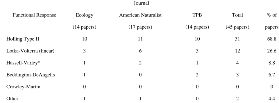
There is a vast literature of ecological theory resting upon the H2 model. I

inspected papers in three leading ecology journals over the past four years (Table 1), and found that 69% of the papers specifying a functional response employ the H2 model. The second-most specified functional response was the linear Lotka-Volterra model, f = aN, as specified in 27% of the papers. In contrast, 7% and 0% of these studies employ the BD and CM models, respectively (two of the three studies employing the BD model are authored by DeAngelis, who introduced the model in 1975).

Four of the papers (9%) in Table 1 specified predator-dependent forms based on the Hassell-Varley model (Hassell and Varley 1969) and similar ratio-dependent forms (forms dependent on N/P rather than N) that have been the subject of many criticisms over the past 10 years (e.g., Abrams 1994, 1997). Because the BD and CM models are mechanistic extensions of the H2 model, I prefer them to the Hassell-Varley model, which was written without a stated mechanistic basis subject to test. However, because of its relatively high profile in the functional response literature, I also include a version of the Hassell-Varley model in my analyses. Also, recently Cosner et al. (1999) have shown that special cases of the Hassell-Varley model (m = 1/3, 1/2, or 1 in Eq. 4, below) can arise from mechanistic assumptions about foraging by spatially grouped predators, and Abrams and Ginzburg (2000) discuss possible mechanistic bases leading to ratio dependence (m = 1).

m

P bN

aN P

N f

+ = ) , (

4 . (4)

Hereafter, I call Eq. 4 the HV model. When m=0 or P=1 the HV model reduces to the H2 model. Arditi and Ackakaya (1990) compared this same model to the H2 model, and found m>0 in each of the ten predator-prey systems they analyzed, hence concluding that the HV model was a better descriptor of the data than the H2 model. They also concluded that ratio-dependent functional responses are likely because most of their confidence intervals for m contain one. When m=1 the HV model depends on N and P only through

the ratio N/P, because Eq. 4 can then be rewritten as f = a⋅(N/P)/(1+b⋅(N/P)).

However, the H2 model’s relative monopoly of the theoretical literature and the debate over ratio dependence (including Arditi and Ackakaya’s results) linger while empirically it remains unclear as to what formthe functional response should take (Abrams and Walters 1996, Murdoch and Briggs 1996, Abrams and Ginzburg 2000). Indeed, Abrams and Walters (1996) conclude, “Although the idea of predator density dependence is very plausible, it is something that has not received much empirical investigation. The literature on ratio-dependent functional responses has yet to produce any conclusive evidence for density dependence of any kind affecting the functional response.”

discriminate among these four alternative functional response models using data sets from 19 simple predator-prey systems.

Methods

I searched the literature via electronic database and literature citations for any study from which I could extract measured instantaneous or integrated feeding rates (defined below) for at least two prey abundances and two predator abundances. I located 19 data sets (Table 2) from 15 sources (14 from the peer-reviewed literature, one Ph.D. dissertation). I did not consider any study that measured a feeding rate but failed to report both predator abundance and prey abundance (e.g., many studies of predator feeding with continuous input of prey; Kennedy and Gray 1993). Some papers reported several similar data sets for the same predator, and in this case I randomly selected one of these data sets so as to include a maximum of one data set per predator-prey system in my analysis. I tested among the four functional response models by first testing each of the three

I analyzed five data sets as representing direct estimates of instantaneous feeding rates, because the author(s) either (i) regularly replaced prey that had been consumed by predators (data sets 2 and 3), or (ii) directly measured the number of prey killed along with predator and prey densities (data sets 1, 4 and 5).

When prey are depleted over the course of the study by predator feeding then integrated feeding rates are measured, and the computations become more cumbersome. In this case, to compare model predictions with the observed data one must integrate the predators’ instantaneous feeding rate over the duration of the empirical study, accounting for prey depletion, resulting in an integrated feeding rate, Fi (i.e.,

P t N N

P N

F_i( (0), )= (0)− ( ) , where N(0) is the initial number of prey and N(t) is the

number of prey remaining after time t). The prey remaining after time t, N(t), is the solution to the appropriate differential equation, where the rate of prey depletion by P predators is

P P N f dt dN

i( , ) −

= , i=1,2,3,4 (5)

for the H2, BD, CM, and HV functional responses, respectively. Predator abundance, P, and initial prey abundance, N(0), are given as the treatment combinations and Eqs. 5 must be solved for the final prey abundance after time t, N(t). These equations can be solved analytically, resulting in an implicit function which must then be solved numerically to find N(t) (Beddington 1975). Alternatively, Eqs. 5 can be numerically integrated to obtain N(t).

Runge-Kutta algorithm; Kincaid and Cheney 1996) to the experimental observations of

integrated feeding rates for different levels of initial prey abundance, N(0), and predator abundance, P, to estimate the parameters a, b, c and m. For the jth observation I assumed the statistical models

(

)

(

)

, , ) , ( log

~ _{i j j wi}

j lognormal f N P

W σ and

(

)

(

)

, , ) ), 0 ( ( log

~ _{i j j yi}

j lognormal F N P

Y σ ,

for instantaneous and integrated measurements of predator feeding rates, respectively (Hilborn and Walters 1992, Carpenter et al. 1994, Pascual and Kareiva 1996, Jost and

Arditi 2000). Here the sets

{

}

j j j

j, , ₌₁and

{

}

n P N Y j j j

j, (0), ₌₁are the observed feeding

rates, prey abundances, and predator abundances from experiments measuring

instantaneous and integrated feeding rates, respectively. The parameter n is the sample

size, and the parameters log(fi(Nj, Pj)) and log(Fi(Nj(0), Pj)), and σw,i2 and σy,i2 are the

expectations and variances of log(Wj) and log(Yj), respectively. I estimated the parameters

a, b, c, and m by maximum likelihood, minimizing the sums of squares

(

)

∑

w W f N P

SS

1

2 , log( ) log( ( , ) ,

for instantaneous feeding rates. The sums of squares for integrated feeding rates is analogous. I estimated the variances using

p n

S

S wi

where p is the number of parameters in the functional response and SˆSw,i is the maximum

likelihood estimate of SS_w,i(Seber and Wild 1989; the variance estimator for integrated

feeding rates is analogous).

To test the BD and CM models against the H2 model I tested whether c=0, because each of the three predator-dependent models reduces to the H2 model when c=0, by computing 95% confidence intervals for c for each of the predator-dependent forms. Similarly, for the HV model, I computed 95% confidence intervals for m, because the HV model reduces to the H2 model for m=0. I computed the 95% confidence intervals by computer simulation (i.e., I employed a parametric bootstrap with 500 bootstrap replicates per model per data set; Efron and Tibshirani 1993, Dennis and Taper 1994).

To test among the alternative predator-dependent forms I used the likelihood-ratio test statistic, defined, for instantaneous feeding rates, for example, as

(

)

i n SS SS

T = −

(the test statistic for integrated feeding rates is analogous). If model i fits the data better than model j, then Ti,j will be positive. Conversely, if model j fits the data better than

model i, then Ti,j will be negative. This test statistic is identical to the difference between

two Akaike Information Criterion (AIC) values for the case of comparing two models with the same number of parameters (Hilborn and Mangel 1997), as is the case here.

here. However, for testing among the three predator-dependent models I do not have justification for specifying any model as the null hypothesis and therefore I employ a test that puts the BD, CM, and HV models on “equal footing” by managing for errors in either direction. Accordingly, I defined the critical values for the test statistic Ti,j as

) , min( 2,

1 , ,j i j i j

i k k

L = and max( , 2, )

1 , ,j i j ij

i k k

U =

where k_i1_{, j} and k_i2_{, j} satisfy

{

}

PrTi,j <ki1,j Hi = and Pr

{

}

2 ,

,j > ij j =

i k H

T ,

where Hi and Hj represent the hypothesized functional responses fi and fj, respectively.

The resulting test is: reject Hi if Ti,j < Li,j, reject Hj if Ui,j < Ti,j , or reject neither Hi or Hj if

Li,j≤ Ti,j≤ Ui,j .

I parameterized the models with 95% confidence intervals for a, b, c and m and computed Li,j and Ui,j by computer simulation (i.e., I used parametric bootstrap to

compute confidence intervals and the distributions of the test statistics using 500

bootstrap replicates per model per data set). I report the outcomes of my hypothesis tests

using the observed values of the test statistic T_iobs_,j , the P-values

{

}

j i j

i