Analysis of Nonlinear Delay Systems with Applications in Bumblebee
Population Models
H.T. Banks∗, J.E. Banks@, Riccardo Bommarco+, A.N. Laubmeier ∗, N.J. Myers ∗, Maj Rundl¨of†, and Kristen Tillman∗
∗Center for Research in Scientific Computation North Carolina State University
Raleigh, NC 27695-8212 USA and
@Undergraduate Research Opportunities Center California State University, Monterey Bay
Seaside, California 93955 and
+Swedish University of Agricultural Sciences Department of Ecology
750 07 Uppsala, Sweden and
†Department of Biology Lund University 223 62 Lund, Sweden
June 3, 2017
Abstract
Bumblebees are ubiquitous creatures and crucial pollinators to a vast assortment of crops worldwide. These populations have been in decline in recent decades and researchers are seeking to understand why populations are decreasing and how to direct conservation efforts. Because of their reproductive patterns, bumblebee population dynamics can be modeled with delay differential equations (DDEs). We present non-linear, non-autonomous DDE models of bumblebee colonies and resources. We demonstrate that the models satisfy the conditions in [4] and complete the subsequent theoretical developments therein in order to rigorously justify families of approximate solutions.
Key words: population models, delay differential equations, non-linear, non-autonomous, spline approximations, Bombus terrestris, reproduction
1
Introduction
The protection of bumblebee populations, among other pollinators, is vital to sustain global agricultural food production [26, 19], biodiversity and ecosystem functioning [18, 30]. It is now widely accepted that bumblebee diversity has dramatically declined in the past several decades [12, 13, 14]. Diminishing populations have been ascribed to habitat loss, resulting in many consequences, including loss of nest and flower resources [32, 41]. The buff-tailed bumblebeeBombus terrestris has been the subject of much study (see for example, [38, 31, 16, 17, 1]), as it is abundant in Europe and known to be an important pollinator [25].
Empirical research has concluded that forage resources (pollen and nectar) in the landscape affect overall bumblebee abundancy. Mathematical modeling based on empirical information on life history parameters can be a strong tool [35, 39, 40] to project population dynamics and identify vulnerable traits and life stages. Such mathematical modeling, especially in an iterative approach [10], can be used for projecting population abundance and understanding the importance of key life traits, such as survival, reproduction and seasonal reproductive switch times under contrasting scenarios. We have used delay differential equations to understand the various ways in which B. terrestris populations are dynamically affected by environmental pressures, including pesticide exposure and resource limitation. In [6, 7], we presented a delay differential equation (DDE) model to simulate the abundance of different bumblebee castes and in-nest resources over time, with dynamics including colony establishment, mortality, colony growth, reproduction, and queen hibernation. Delay equations have been used in various applications, including biology, ecology, engineering (see [2, 15, 20, 23] for examples) and even honeybee population modeling [24]. We refer the reader to [37] for an introduction to DDEs and applications, as well as [27] for DDEs in ecology. In [6, 7], we explained why a DDE model may be preferable over the more commonly used ordinary differential equation (ODE) system for describing bumblebee and other population dynamics. In addition, we presented several models with the underlying assumptions and proposed ways in which pressures such as resource limitation and insecticide exposure can be reflected in the model. We also described a linear spline approximation method for obtaining numerical solutions to our models and provided model simulations in the absence of pressures. Here, we demonstrate that the models in [6, 7] satisfy the assumptions required in [4], and complete the necessary theory in order to obtain the approximate solution to the DDE system. The theory we complete here, first outlined in detail in [4] without proofs, has subsequently been discussed or referred to in various publications [3, 5, 8, 9, 28, 29, 33, 34] in the past 35 years, but proofs for the outline in [4] have not been presented. Since not all of the references cited above are readily accessible (including [4] itself), we present here the complete theory and verify that our models from [6, 7] satisfy the theory.
2
Models
2.1 Bumblebee DDE models
We present a general bumblebee model, versions of which were originally discussed in [6, 7], and which is 6-dimensional with state variables: in-nest nectar abundance A(t), in-nest pollen abundance B(t), queens Q(t), workers W(t), males M(t) and gynes (daughter queens) G(t). The version discussed here has been slightly modified from those developed in [6, 7] and is currently being used in pesticide studies. We define the first day of spring, when hibernating gynes emerge as new queens that found new colonies, at t=TS. We therefore consider
whereTW is the end of the season. The dynamics of a collection of hives are described by the DDE
dA
dt = (bAW −µAW)W −µAQQ−2 [lW(t, Qt) +lM(t, Qt) +lG(t, Qt)] dB
dt = (bBW −µBW)W −µBQQ−[lW(t, Qt) +lM(t, Qt) +lG(t, Qt)] dQ
dt =−µQQ dW
dt =bW(t−22)Q(t−22)SW(t, At, Bt, Wt)−µWW dM
dt =bM(t−26)Q(t−26)SM(t, At, Bt, Wt)−µMM dG
dt =bG(t−30)Q(t−30)SG(t, At, Bt, Wt)−µGG with initial conditions and histories forθ∈[−30,0],
ATS+22(θ) =A0 WTS+22(θ) =
0 θ <0 W0 θ= 0 BTS+22(θ) =B0 MTS+22(θ) = 0
QTS+22(θ) =Q0e
−µQ(TS+22+θ) G
TS+22(θ) = 0.
As is usual in the formulation of delay equations, the notationQt, etc., refers to the functionQt(θ) =Q(t+θ), θ∈
[−30,0], etc. Larval consumption in the equations for dAdt and dBdt is modelled as
lW(t, Qt) =
Z t−4
t−13
bW(s)Q(s)P0er¯(t−s)ds,
lM(t, Qt) =
Z t−4
t−15
bM(s)Q(s)P0er¯(t−s)ds,
lG(t, Qt) =
Z t−4
t−17
bG(s)Q(s)P0e¯r(t−s)ds,
where ¯r is a larval pollen consumption growth rate. The birth rates of workers, males, and gynes depend on predefined seasonal switch times T∗ and T∗∗; in formulating these terms, we enforce the conditions that for t < T∗∗, bM(t), bG(t) = 0 and for t > T∗∗, bW(t) = 0. The probabilities of survival for worker, male, and gyne
larvae are given by
SW(t, At, Bt, Wt) =
1 9
Z t−9
t−18 L
W(s) γWQ(s)
L
A(s) AmaxQ(s)
L
B(s) BmaxQ(s)
ds,
SM(t, At, Bt, Wt) =
1 11
Z t−11
t−22 L
W(s) γMQ(s)
L
A(s) AmaxQ(s)
L
B(s) BmaxQ(s)
ds,
SG(t, At, Bt, Wt) =
1 13
Z t−13
t−26 L
W(s) γGQ(s)
L
A(s) AmaxQ(s)
L
B(s) BmaxQ(s)
ds,
for the function
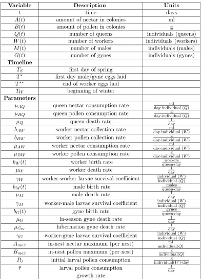
Variable Description Units
t time days
A(t) amount of nectar in colonies ml
B(t) amount of pollen in colonies g
Q(t) number of queens individuals (queens) W(t) number of workers individuals (workers)
M(t) number of males individuals (males)
G(t) number of gynes individuals (gynes)
Timeline
TS first day of spring
T∗ first day male/gyne eggs laid T∗∗ end of worker eggs laid TW beginning of winter
Parameters
µAQ queen nectar consumption rate day·individual (ml Q)
µBQ queen pollen consumption rate day·individual (g Q)
µQ queen death rate day1
bAW worker nectar collection rate day·individual (ml W)
bBW worker pollen collection rate day·individual (g W) µAW worker nectar consumption rate day·individual (ml W)
µBW worker pollen consumption rate day·individual (g W) bW(t) worker birth rate queen·dayworkers
µW worker death rate day1
γW worker-worker larvae survival coefficient individual (individual (WQ))
bM(t) male birth rate queen·daymales
µM male death rate day1
γM worker-male larvae survival coefficient individual (individual (WQ))
bG(t) gyne birth rate queen·daygynes
µG in-season gyne death rate day1
µGW hibernation gyne death rate
1 day γG worker-gyne larvae survival coefficient individual (individual (WQ))
Amax in-nest nectar maximum (per nest) individual(ml Q)
Bmax in-nest pollen maximum (per nest) individual(g Q)
P0 initial larval pollen consumption individual(g W)·day ¯
r larval pollen consumption day1
growth rate
2.2 General formulation and hypothesis
Now, consider the following DDE form, as given in [4]: dx
dt =f(t, x(t), xt, x(t−τ1), ..., x(t−τν)) +f2(t), x0 =φ,
(2)
for 0≤t≤T andf : [0, T]×Z×Rn×ν →
Rn. We defineZ =Rn×L2(−r,0), 0< τ1< ... < τν =r,xt(θ) =x(t+θ)
for −r ≤ θ≤0. We assume that φ∈ H1(−r,0) (whereHj(a, b) denotes the Sobolev space Wj,2(a, b,Rn) of Rn
-valued functions f such that f ∈L2[a, b], ∂jf ∈L2[a, b] ), andf2 ∈L2(0, T). We further assume that f satisfies the hypotheses from [4]:
(H1) The functionf satisfies a global Lipschitz condition
f(t, η, ψ, y1, ..., yν)−f(t, ξ,
˜
ψ, w1, ..., wν)
Rn
≤K ||η−ξ||
Rn+
ψ−
˜ ψ
L2(−r,0)+
ν
X
i=1
||yi−wi||Rn
!
for some fixed constant K and all (t, η, ψ, y1, ..., yν),(t, ξ,ψ, w˜ 1, ..., wν) ∈Rn×Z ×Rn×ν. (A more relaxed
condition would also suffice, in which K = K(t), some uniformly bounded function on the interval [0, T]). We proceed with the assumption thatK is constant.
(H2) The functionsf2 : [0, T]→Rnandf : [0, T]×Z×Rn×ν →Rnare differentiable with all derivatives (ordinary
and partial) dominated by integrable functions.
We define x= [A, B, Q, W, M, G]T. Then the system DDE can be written as
dx
dt =f(t,x(t),xt,x(t−22),x(t−26),x(t−30)),
=
fA(t,x(t),xt,x(t−22),x(t−26),x(t−30))
fB(t,x(t),xt,x(t−22),x(t−26),x(t−30))
fQ(t,x(t),xt,x(t−22),x(t−26),x(t−30))
fW(t,x(t),xt,x(t−22),x(t−26),x(t−30))
fM(t,x(t),xt,x(t−22),x(t−26),x(t−30))
fG(t,x(t),xt,x(t−22),x(t−26),x(t−30))
.
We note here that the the subscriptsA, B, Q, ..., etc., are used to denote the components of theRn=R6 function
f. We can see from the model statement that (H2) is satisfied for the bumblebee DDE. We proceed to show that the Lipschitz condition (H1) is satisfied for the bumblebee model
2.3 Lipschitz condition for the bumblebee model
We introduce the notation that for a function f(t,x(t),xt,x(t−22),x(t−26),x(t−30)),
δf =f(t,x˜(t),x˜t,x˜(t−22),x˜(t−26),x˜(t−30))−f(t,x(t),xt,x(t−22),x(t−26),x(t−30)),
and note that ||δf||2
R6 =δfA
2+δf2
B+δfQ2 +δfW2 +δfM2 +δfG2.
bW,max. Then by noting that the integrand in the larval consumption term is non-negative, we have
(lW(t, Qt)−lW(t,Q˜t))2 =
Z t−4
t−13
bW(s)Q(s)P0e¯r(t−s)ds−
Z t−4
t−13
bW(s) ˜Q(s)P0er¯(t−s)ds
2
=≤9
Z t−4
t−13
bW(s)[Q(s)−Q(s)]P˜ 0er¯(t−s)
2
ds
≤9
Z t
t−30
bW(s)[Q(s)−Q(s)]P˜ 0e¯r(t−s)
2
ds
≤9b2W,maxP02e60r
Z t
t−30
[Q(s)−Q(s)]˜ 2ds.
Similar inequalities forlM andlG can be obtained under the assumption that there exist finite constants such that
bM(t)≤bM,max and bG(t)≤bG,max for all t. ForKl= 18P0e30rmax(bW,max, bM,max, bG,max), we obtain
δfA2 ≤3(bAW −µAW)2(W(t)−W˜(t))2+ 3µ2AQ(Q(t)−Q(t))˜ 2+ 3Kl2
Z t
t−30
[Q(s)−Q(s)]˜ 2ds
≤3(bAW −µAW)2(W(t)−W˜(t))2+ 3µ2AQ(Q(t)−Q(t))˜ 2+ 3Kl2||xt−x˜t||2L2.
Similarly,
δfB2 ≤3(bBW −µBW)2(W(t)−W˜(t))2+ 3µ2BQ(Q(t)−Q(t))˜ 2+ 3(Kl/2)2||xt−˜xt||2L2.
The function L(x) of (1) satisfies the Lipschitz condition,
L(x)−L(˜x) = 1−e −x
1 +e−x −
1−e−˜x 1 +e−˜x =
(1−e−x)(1 +e−˜x)−(1−e−˜x)(1 +e−x) (1 +e−x)(1 +e−˜x)
≤(1−e−x)(1 +e−˜x)−(1−e−˜x)(1 +e−x) = 2(e−˜x−e−x)≤2|x−x˜|. Moreover, since L(x)∈[0,1] for allx >0, we have for positive arguments
L(x)L(y)L(z)−L(˜x)L(˜y)L(˜z) = [L(x)−L(˜x)]L(y)L(x) + [L(y)−L(˜y)]L(˜x)L(z) + [L(˜z)−L(z)]L(˜x)L(˜y)
≤2|x−x˜|+ 2|y−y˜|+ 2|z−z˜|. Thus we find that the worker survivability term satisfies the inequality
δSW ≤
1 9
Z t−9
t−18 2
W(s) γWQ(s)
− W˜(s)
γWQ(s)˜
+ 2
A(s) AmaxQ(s)
− A(s)˜
AmaxQ(s)˜
+ 2
B(s) BmaxQ(s)
− B(s)˜
BmaxQ(s)˜
ds.
We note that the solution Q(s) is exponentially decreasing, so Q(s) is bounded above by Q0 and below by KQ = Q0e−µQ(TW−TS−22) for all s. Then for KW = W0ebW,maxQ0(TW−TS−22), we have W(s) ≤KW for all s. We
therefore have
W(s) γWQ(s)
− W˜(s)
γWQ(s)˜
= 1 γW
W(s) ˜Q(s)−W˜(s)Q(s) Q(s) ˜Q(s)
≤ 1
γWKQ2
W(s) ˜Q(s)−
˜
W(s)Q(s)
≤ 1
γWKQ2
˜ Q(s)
W(s)−
˜ W(s)
+
˜ W(s)
Q(s)−
˜ Q(s)
≤ 1
γWKQ2
Q0
W(s)−W˜(s)
+KW
Q(s)−Q(s)˜
By similarly noting that for KA=A0e(bAW−µAW)KW(TW−TS−22) and KB =B0e(bBW−µBW)KW(TW−TS−22), we have A(s)≤KA and B(s)≤KB for alls, we obtain
δSW2
≤
2 9
Z t−9
t−18
W(s)−W˜(s)
γWKQ2/Q0 +
A(s)−A(s)˜
AmaxKQ2/Q0 +
B(s)−B(s)˜
BmaxKQ2/Q0
+KW +KA+KB γWKQ2
Q(s)−Q(s)˜ ds 2 ≤4 81 Z t t−30
W(s)−W˜(s)
γWKQ2/Q0 +
A(s)−A(s)˜
AmaxKQ2/Q0 +
B(s)−B(s)˜
BmaxKQ2/Q0 +
KW
γW +
KA
Amax +
KB Bmax K2 Q
Q(s)−Q(s)˜ ds 2 ≤120 81 Z t t−30
W(s)−
˜ W(s)
γWKQ2/Q0 + A(s)− ˜ A(s)
AmaxKQ2/Q0 +
B(s)−
˜ B(s)
BmaxKQ2/Q0 +
KW
γW +
KA
Amax +
KB
Bmax
KQ2
Q(s)− ˜ Q(s) 2 ds ≤840 81 Z t t−30
W(s)−
˜ W(s)
(γWKQ2/Q0)2 2 + A(s)− ˜ A(s)
(AmaxKQ2/Q0)2 2
+
B(s)−
˜ B(s)
(BmaxKQ2/Q0)2 2
+(
KW
γW +
KA
Amax +
KB
Bmax)
2
(KQ2)2
Q(s)− ˜ Q(s) 2 ds ≤280 27 max Q0 γWKQ2
, Q0 AmaxKQ2
, Q0 BmaxKQ2
,
KW
γW +
KA
Amax +
KB
Bmax
KQ2
!2
||xt−˜xt||2L2.
In the second to last inequality above we have used the easily verifiable inequality (a+b+c+d)2 ≤7(a2+b2+c2+d2). Computing the quantityδfW2 , we find
δfW2 = (bW(t−22)Q(t−22)SW(t, At, Bt, Wt, Qt)−µWW(t)
−bW(t−22) ˜Q(t−22)SW(t,A˜t,B˜t,W˜t,Q˜t) +µWW˜(t)
2
= 2bW(t−22)2
Q(t−22)δSW +S(t,A˜t,B˜t,W˜t)(Q(t−22)−Q(t˜ −22)
2
+ 2µ2W( ˜W(t)−W(t))2
≤4b2W,maxQ20δSW2 + 4b2W,max
Q(t−22)−
˜
Q(t−22)
2
+ 2µ2W
W(t)−
˜ W(t) 2
≤KSW ||xt−˜xt||
2
L2 + 4b
2
W,max||x(t−22)−x˜(t−22)||
2 R6+ 2µ
2
W
W(t)−W˜(t)
2 ,
whereKSW =
1120 27 b
2
W,maxQ20max
Q0 γWK2Q
,A Q0
maxKQ2,
Q0 BmaxKQ2 ,
KW γW + KA Amax+ KB Bmax K2 Q 2 . We similarly have
δfM2 ≤KSM ||xt−˜xt||
2
L2 + 4b2M,max||x(t−26)−x˜(t−26)||2R6 + 2µ2M
M(t)−
˜ M(t) 2
forKSM =
3360
121b2M,maxQ20max
Q0 γMKQ2,
Q0 AmaxKQ2,
Q0 BmaxK2Q,
KW γM + KA Amax+ KB Bmax K2 Q 2 and
δfG2 ≤KSG||xt−˜xt||
2
L2 + 4b
2
G,max||x(t−30)−x˜(t−30)||
2 R6 + 2µ
2
G
G(t)−G(t)˜
2
forKSG=
3360 169 b
2
G,maxQ20max
Q0 γGKQ2
,A Q0
maxK2Q
,B Q0
maxKQ2
,
KW
γG +AmaxKA +BmaxKB
K2
Q
2
We note thatδfQ2 =µ2Q(Q−Q)˜ 2. Combining the above expressions, we obtain
||δf||2
R6 ≤K1||x(t)−x˜(t)|| 2
R6 +K2||xt−˜xt|| 2
L2+K3
3
X
i=1
||x(t−τi)−x˜(t−τi)||2R6,
for delaysτ1 = 22, τ2= 26, τ3 = 30 and constants K1= max
3(bAW −µAW)2,3µ2AQ,3(bBW −µBW)2,3µ2BQ,2µW2 ,2µ2M,2µ2G
,
K2= max
3Kl2, KSW, KSM, KSG
,
K3= max
4b2W,max,4b2M,max,4b2G,max
.
Then, taking K= max(√K1,
√
K2,
√
K3), we have the Lipschitz condition
||δf||
R6 ≤K ||x(t)−x˜(t)||R6 +||xt−˜xt||L2+ 3
X
i=1
||x(t−τi)−x˜(t−τi)||R6
!
3
Theoretical developments of solution approximations
3.1 Notation and preliminary background
In [4] (see also a summary in [5]), the author presents the development of solutions for a general class of spline approximations to nonlinear functional differential equations. As stated in Section 2.1, we consider problems of the form (2) satisfying conditions (H1) and (H2). We next carry out discussions of underlying proofs of Theorems 2.1 and 2.2 and the supporting Lemmas 2.2-2.6 cited in [4]. We first introduce the necessary notation and some preliminary results.
We define the function F : [0, T]×Z →Rnby
F(t, η, ψ) =f(t, η, ψ, ψ(−τ1), ..., ψ(−τν)), (3)
and we define the nonlinear operatorA(t) :D(A)⊂Z →Z by
D(A) =W ≡ {(ψ(0), ψ)ψ∈H1(−r,0)},
A(t)(ψ(0), ψ) = (F(t, ψ(0), ψ), ψ0).
We let ZN be the approximating linear spline subspace (see [8, 4, 5]) of Z such that
ZN =(φ(0), φ)| φa continuous, linear spline with nodes attNi =−ir/N, j= 0,1, ..., N , and PN =PgN be the orthogonal projection inh·,·ig ofZ onto ZN, where
h(ψ(0), ψ),( ˜ψ(0),ψ)˜ ig =hψ(0),ψ(0)˜ iRn+
Z 0
−r
hψ(σ),ψ(σ)˜ iRng(σ)dσ
forg the linear weighting function defined on [−r,0] given by
g(ξ) =j for ξ ∈[−τν−j+1,−τν−j], j = 1,2, ..., ν.
We recall [8, 5] that the associated norm || · ||g generates a topology onZ =Rn×L2(−r,0) that is equivalent to theZ topology. Furthermore, all of the usual density results involving the spacesHj(−r,0) hold in the equivalent topology onZ as well as in the standardRn×L2 topology.
We restate Lemma 2.1 of [4], which will be of use in Section 3.2 below.
Lemma 2.1. If X is a Hilbert space and x: [a, b]→X is given byx(t) =x(a) +Raty(σ)dσ, then
||x(t)||2 =||x(a)||2+ 2
Z t
0
hx(σ), y(σ)idσ. (4)
Lemma 2.1 is a restatement of a well-established equality (see [11, p. 100]) which follows immediately from d
dt 1 2
x(t)2
=hx(t), x(t)˙ i.
We will also utilize the integral form of Gronwall’s Inequality for continuous functions [21], as stated below.
Gronwall’s Inequality. Let I be an interval in R ( [a,∞),[a, b] or [a, b) with a≤b ). Let α, β, and u be
real-valued functions onI with the following conditions: β andu are continuous, the negative part ofα is integrable on every closed, bounded subinterval ofI,β is non-negative,αis non-decreasing, and usatisfies the integral inequality
u(t)≤α(t) +
Z t
a
β(σ)u(σ)dσ ∀t∈I.
Then
u(t)≤α(t)e
Rt
Finally, we will use the following inequality for inner products on Banach spaces. Ifx, yare elements of a Banach space, then
hx, yi ≤ 1
2(||x||
2+||y||2) (5)
where|| · || is the norm induced by the inner product.
3.2 Theoretical Developments
We next discuss arguments underlying proofs of a series of theorems and lemmas.
Theorem 2.1. Assume that (H1) holds and let z(t;φ, f2) = (x(t;φ, f2), xt(φ, f2)), where x is the solution of (2) corresponding to φ∈H1, f2∈L2. Then for ζ = (φ(0), φ), z(t;φ, f2) is the unique solution on [0, T]of
z(t) =ζ+
Z t
0
[A(σ)z(σ) + (f2(σ),0)]dσ. (6)
Furthermore, f2→z(t;φ, f2) is weakly sequentially continuous from L2 (weak) to Z (strong).
This is precisely Theorem 2.1 of [4]. The existence part of the proof is based on a standard uniform contraction principle [22, p. 7] well known to investigators of dynamical systems in the 1970’s and 1980’s. Earlier versions of Theorem 2.1 for linear delay systems are given in [3, 33, 34]. The theorem is stated as Theorem 2.1 in [29]. A detailed proof (which we will not repeat here) is given in [28]. To prove solution uniqueness, we make use of the dissipative inequality stated and proved below.
DDE Dissipative Inequality: Forz, z∈ D(A),
hA(t)z− A(t)z, z−zig ≤w(t)||z−z||2g. (7)
To establish this inequality, we letz= (φ(0), φ) and z= (φ(0), φ), z, z∈ D(A). Then by definition ofA, we have
hA(t)z− A(t)z, z−zig=h(F(t, φ(0), φ), φ0)−(F(t, φ(0), φ), φ
0
),(φ(0), φ)−(φ(0), φ)ig
=h(F(t, φ(0), φ)−F(t, φ(0), φ), φ0−φ0),(φ(0)−φ(0), φ−φ)ig
=hF(t, φ(0), φ)−F(t, φ(0), φ), φ(0)−φ(0)iRn+
Z 0
−r
hφ0(σ)−φ0(σ), φ(σ)−φ(σ)iRng(σ)dσ.
(8)
By (H1), we have
hF(t, φ(0), φ)−F(t, φ(0), φ), φ(0)−φ(0)iRn ≤
F(t, φ(0), φ)−F(t, φ(0), φ)
Rn
φ(0)−φ(0)
Rn
≤K
φ(0)−φ(0)
Rn+
φ−φ
L2(−r,0)+
ν
X
i=1
φ(−τi)−φ(−τi)
Rn
!
φ(0)−φ(0)
Rn.
By definition ofg, the second term in the inner product in (8) is
Z 0
−r
hφ0(σ)−φ0(σ), φ(σ)−φ(σ)iRng(σ)dσ=
Z 0
−r
d dσ
hφ(σ)−φ(σ), φ(σ)−φ(σ)iRn
2
g(σ)dσ
=
ν
X
i=1
Z −τi−1
−τi
d dσ
φ(σ)−φ(σ)
2 Rn 2
!
(ν+ 1−i)dσ
=
ν
X
i=1
(ν+ 1−i)
φ(−τi−1)−φ(−τi−1)
2 Rn
2 −
φ(−τi)−φ(−τi)
2 Rn 2
!
= ν 2
φ(0)−φ(0)
2 Rn−
ν
X
i=1
φ(−τi)−φ(−τi)
2 Rn
Substitution yields
hA(t)z− A(t)z, z−zig ≤(K+
ν 2)
φ(0)−φ(0)
2 Rn+K
φ−φ
L2(−r,0)
φ(0)−φ(0) Rn + ν X i=1 K
φ(−τi)−φ(−τi) Rn
φ(0)−φ(0)
Rn−
φ(−τi)−φ(−τi) 2 Rn 2
≤(K+ν 2)
φ(0)−φ(0)
2 Rn+K
φ−φ 2
L2(−r,0)
2 +
φ(0)−φ(0) 2 Rn 2 + ν X i=1
φ(−τi)−φ(−τi) 2 Rn 2 +
φ(0)−φ(0)
2 RnK
2 2 ! −
φ(−τi)−φ(−τi) 2 Rn 2
= (K+ν 2 +
K 2 +
K2ν 2 )
φ(0)−φ(0)
2 Rn+
K 2 φ−φ 2
L2(−r,0)
≤ ν 2 + 3K 2 +
K2ν 2
φ(0)−φ(0)
2 Rn+
φ−φ 2
L2(−r,0)
.
We definew(t) =
ν
2 + 3K
2 +
K2ν
2
and note that becauseg(σ)≥0 for allσ ∈[−r,0] we have
φ(0)−φ(0)
2 Rn+
φ−φ 2
L2(−r,0) ≤ ||z−z|| 2
g.
The dissipative inequality hA(t)z− A(t)z, z−zig ≤w(t)||z−z||2g therefore holds.
To establish the desired uniqueness of solutions to equation (6), we let φ, φ∈H1(−r,0) and define ζ = (φ(0), φ) and ζ = (φ(0), φ). Then the corresponding solutions to (6) are given by
z(t) =ζ+
Z t
0
[A(σ)z(σ) + (f2(σ),0)]dσ,
z(t) =ζ+
Z t
0
[A(σ)z(σ) + (f2(σ),0)]dσ.
Supposeζ =ζ. Then we have
z(t)−z(t) =
Z t
0
[A(σ)z(σ)− A(σ)z(σ)]dσ.
Application of Lemma 2.1, the dissipative inequality (7), and Gronwall’s Inequality yields
||z(t)−z(t)||2g ≤2
Z t
0
hA(σ)z(σ)− A(σ)z(σ), z(σ)−z(σ)igdσ
≤2
Z t
0
w(σ)||z(σ)−z(σ)||2gdσ≤0·exp
Z t
0
2w(σ)dσ
= 0.
We therefore have z(t) =z(t) and the solution to (6) is unique.
LetZN andPN =PgN be the linear spline subspaces and projections as defined above. For the approximating operatorAN(t) =PNA(t)PN, we define the approximating solutions inZN
zN(t) =PNζ+
Z t
0
[AN(σ)zN(σ) +PN(f2(σ),0)]dσ, (9)
which are the unique solutions of the differential equation dzN
dt =A
N(t)zN(t) +PN(f
2(t),0), zN(0) =PNζ.
We note that these equations are finite dimensional ordinary differential equations and hence existence of solutions are readily guaranteed. To prove uniqueness, we will make use of the following dissipative inequality.
Approximation Dissipative Inequality: Forz, z ∈ D(A),
hAN(t)z− AN(t)z, z−zig≤w(t)||z−z||2g. (11)
By definition ofAN and (7), we have
hAN(t)z− AN(t)z, z−zig =hPNA(t)PNz−PNA(t)PNz, z−zig
≤ hA(t)PNz− A(t)PNz, PNz−PNzig ≤w(t)
PNz−PNz
2
g≤w(t)||z−z||
2
g.
Now, let φ, φ∈H1(−r,0) and define ζ = (φ(0), φ) and ζ = (φ(0), φ). Then the corresponding solutions to (9) are given by
zN(t) =PNζ+
Z t
0
[AN(σ)zN(σ) +PN(f2(σ),0)]dσ,
zN(t) =PNζ+
Z t
0
[AN(σ)zN(σ) +PN(f
2(σ),0)]dσ.
Supposeζ =ζ. Then we have
zN(t)−zN(t) =
Z t
0
[AN(σ)zN(σ)− AN(σ)zN(σ)]dσ.
Application of Lemma 2.1, and (11) (noting that ZN ⊂ D(A)), and Gronwall’s Inequality yields
zN(t)−zN(t)
2
g ≤2
Z t
0
hAN(σ)zN(σ)−AN(σ)zN(σ), zN(σ)−zN(σ)igdσ
≤2
Z t
0
w(σ)
zN(σ)−zN(σ)
2
gdσ≤0·exp
Z t
0
2w(σ)dσ
= 0.
Theorem 2.3. Assume (H1), (H2). Let ζ = (φ(0), φ), φ ∈ H1 and f2 ∈ H0(0, T) be given, with zN and z the corresponding solutions on [0, T] of (10) and (6) respectively. Then zN(t) → z(t) = (x(t;φ, f2), xt(φ, f2)) as N → ∞, uniformly int on [0, T].
The proof of this theorem follows from the Lemmas below.
Lemma 2.2. Assume (H1) and let Z = {z = (φ(0), φ)|φ ∈ H2}. Then AN(t)z → A(t)z as N → ∞ for each
z∈ Z. Proof:
For z= (φ(0), φ) and corresponding approximationPNz= (PNφ(0), PNφ), we consider the quantity
AN(t)z− A(t)z
g. Applying the definition ofA
N (and suppressing the dependence on t), we have
ANz− Az
g =
PNAPNz− Az
g =
PNAPNz−PNAz+PNAz− Az
g
≤
PNAPNz−PNAz
g+
PNAz− Az
g.
(12)
However, PNAz→ Az asN → ∞. We additionally note that
PNAPNz−PNAz
g ≤
APNz− Az
By definition of the operator Aand theg-norm, we have
APNz− Az
2
g=
(f(t, PNφ(0), PNφ),(PNφ)0)−(f(t, φ(0), φ), φ0)
2
g
=
f(t, PNφ(0), PNφ)−f(t, φ(0), φ)
2 Rn+
Z 0
−r
(PNφ)0(σ)−φ0(σ)
2
Rng(σ)dσ.
(13)
By (H1),
f(t, PNφ(0), PNφ)−f(t, φ(0), φ)
Rn
≤K
PNφ(0)−φ(0)
Rn+
PNφ−φ
L2(−r,0)+
ν
X
i=1
PNφ(−τi)−φ(−τi)
Rn
!
. (14)
But from Theorems 2.5 and 2.6 of [36], we have that forφ∈H2(−r,0), (PNφ)0−φ0 →0 inL2g and PNφ−φ→0 pointwise on [−r,0] as well as inL2g.
Lemma 2.3. Let T ={(ζ, f2) ∈ W ×H0(0, T) =D(A)×L2(0, T) |φ ∈H2(−r,0), f2 ∈H1(0, T), with ˙φ(0) = F(0, ζ) +f2(0) whereζ = (φ(0), φ)}. Assume that (H1), (H2) hold. Then for (ζ, f2) ∈ T, the corresponding solution σ→z(σ) = (x(σ), xσ) of (6) (wherex is the solution of (2)) satisfies z(σ)∈ Z for each σ ∈[0, T]).
Proof:
Recall that xσ(τ) =x(σ+τ) for τ ∈[−r, T−τ]. Assume (H1), (H2). Let (ζ, f2)∈ T andσ ∈[0, T]. We want to show that z(σ) ∈ Z = {(x(σ), xσ)|xσ ∈ H2(−r, T −τ)}. It is enough to show that x(σ) ∈ Rn, xσ,x˙σ,x¨σ ∈
L2(−r, T−τ), wherexis the solution of (2) (see Theorem 2.1). Clearly,x(σ)∈Rnbecausef : [0, T]×Z×Rnν →Rn.
Furthermore,xσ ∈L2(−r, T−τ) ⇐⇒ xσ is integrable and real-valued on [−r, T −τ] and
||xσ||2=
Z T−τ
−r
|xσ(t)|2dt
1/2
<∞.
By definition ofF,xσ is continuous and real-valued on [−r, T−τ].Because [−r, T−τ] is a finite interval, we have
||xσ||2 <∞. Therefore xσ ∈L2[−r, T−τ]. The first derivative ˙xσ(t) has history ˙ζ= ( ˙φ(0),φ) with˙ φ∈H2(−r,0)
and
˙
φ(0) =F(0, ζ) +f2(0) =f(0, φ(0), φ, φ(−τ1), . . . , φ(−τν)) +f2(0).
Withφ∈H2(−r,0), we have ˙φ∈L2(−r,0), and ˙φis continuous and real valued on [−r,0]. By definition ofF, we have continuity of ˙xacross t= 0. Therefore ˙xσ is continuous on [−r, T −τ] and thus we find ||x˙σ||2 <∞.
Finally,φ∈H2(−r,0)⇒φ¨∈L2, so ¨φis integrable and real-valued on [−r,0]. By definition of ˙φfor (ζ, f2)∈ T, we have
¨
φ(0−) = ˙F(0+, ζ) + ˙f2(0+) = ˙f(0+, φ(0+), φ, φ(−τ1), . . . , φ(−τν)) + ˙f2(0+).
Since f and f2 are differentiable with dominated partial derivatives forf and derivative forf2 on [0, T], we have integrability of ¨φacross t= 0. Therefore ¨xσ is real-valued and integrable on [−r, T −τ] and thus ||x¨σ||2 <∞. Lemma 2.4. Assume (H1), (H2) and let (ζ, f2)∈ T withzN and zthe respective solutions to (9) and (6). Then zN(t)→z(t) uniformly in ton [0, T].
Proof:
Let φ ∈H1(−r,0), f
2 ∈L2(0, T), and define ζ = (φ(0), φ). Denote the solution to (6) for arguments {ζ, f2} as z(t) and the corresponding approximating solution given by (9) as zN(t). We consider the quantity ∆N(t) = zN(t)−z(t), or
∆N(t) = (PN−I)ζ+
Z t
0
By Lemma 2.1, we have
∆N(t)
2 g =
(PN −I)ζ
2 Rn+ 2
Z t
0
hAN(σ)zN(σ)− A(σ)z(σ) + (PN −I)(f2(σ),0),∆N(σ)igdσ
=
(PN −I)ζ
2 Rn+ 2
Z t
0
hAN(σ)zN(σ)− AN(σ)z(σ) +AN(σ)z(σ)− A(σ)z(σ),∆N(t)igdσ
+ 2
Z t
0
h(PN −I)(f2(σ),0),∆N(σ)igdσ
=
(PN −I)ζ
2 Rn+ 2
Z t
0
hAN(σ)zN(σ)− AN(σ)z(σ),∆N(σ)i gdσ
+ 2
Z t
0
hAN(σ)z(σ)− A(σ)z(σ),∆N(σ)igdσ+ 2
Z t
0
h(PN−I)(f2(σ),0),∆N(σ)igdσ.
By (11), we obtain
2
Z t
0
hAN(σ)zN(σ)− AN(σ)z(σ),∆N(σ)igdσ≤2
Z t
0
w(σ) ∆N(σ)
2 gdσ
and by (5), we find
2
Z t
0
hAN(σ)z(σ)− A(σ)z(σ),∆N(σ)igdσ≤
Z t
0
AN(σ)z(σ)− A(σ)z(σ) 2 g+ ∆N(σ)
2 gdσ 2 Z t 0
h(PN −I)(f2(σ),0),∆N(σ)igdσ≤
Z t
0
(PN −I)(f2(σ),0) 2 g+ ∆N(σ)
2 gdσ. Substitution yields ∆N(t)
2 g ≤
(PN −I)ζ
2 Rn+
Z t
0
AN(σ)z(σ)− A(σ)z(σ)
2
gdσ+
Z t
0
(PN −I)(f2(σ),0) 2 gdσ + 2 Z t 0
(ω+ 1) ∆N(σ)
2 gdσ ≤
(PN −I)ζ
2 Rn+
Z T
0
AN(σ)z(σ)− A(σ)z(σ)
2
gdσ+
Z T
0
(PN −I)(f2(σ),0)
2 gdσ + 2 Z t 0
(ω+ 1) ∆N(σ)
2 gdσ
=1(N) +2(N) +3(N) + 2
Z t
0
(w+ 1) ∆N(σ)
2 gdσ for
1(N) =
(PN −I)ζ
2 Rn, 2(N) =
Z T
0
AN(σ)z(σ)− A(σ)z(σ) 2 gdσ,
3(N) =
Z T
0
(PN −I)(f2(σ),0) 2 gdσ.
Then, by Gronwall’s Inequality, we have
∆N(t)
2
g ≤[1(N) +2(N) +3(N)] exp
2
Z t
0
(w(σ) + 1)dσ
Observing that exph2Rt
0(w(σ) + 1)dσ
i
is bounded for t∈[0, T], we find that it suffices to prove that i(N)→0,
i=1,2,3. We have that the convergence of 1 and 3 to 0 is immediately argued while a consideration of Lemma 2.2 along with reference to Theorems 2.5 and 2.6 of [36] reveals that the convergence of AN(σ)z(σ) → A(σ)z(σ)
is dominated on the interval [0, T] and hence we also have 2→0.
Lemma 2.5. Assume (H1). Then the solutions of (6) and (9) depend continuously (in theZ×H0 topology) on (ζ, f2) in W ×H0, uniformly int on [0, T].
Proof:
Let φ, φ ∈ H1(−r,0) and f
2, f2 ∈ L2(0, T) and define ζ = (φ(0), φ) and ζ = (φ(0), φ). Then for arguments
{ζ, f2} and{ζ, f2} denote solutions to (6) asz(t) andz(t) respectively. We define the quantity ∆(t) =z(t;ζ, f2)−z(t;ζ, f2)
and by definition of solutionsz(t), z(t) we obtain
∆(t) =ζ+
Z t
0
[A(σ)z(σ) + (f2(σ),0)]dσ−
ζ+
Z t
0
[A(σ)z(σ) + (f2(σ),0)]dσ
=ζ−ζ+
Z t
0
[A(σ)z(σ)− A(σ)z(σ) + (f2(σ)−f2(σ),0)]dσ=δ1(0) +
Z t
0
δ2(σ)dσ
forδ1(0) =ζ−ζ= (φ(0)−φ(0), φ−φ) and δ2(σ) =A(σ)z(σ)− A(σ)z(σ) + (f2(σ)−f2(σ),0). By Lemma 2.1, we therefore have
h∆(t),∆(t)ig =hδ1(0), δ1(0)ig+ 2
Z t
0
h∆(σ), δ2(σ)igdσ=hδ1(0), δ1(0)ig+ 2
Z t
0
hδ2(σ),∆(σ)igdσ
= ζ−ζ 2
g+ 2
Z t
0
hA(σ)z(σ)−A(σ)z(σ),∆(σ)ig+h(f2(σ)−f2(σ),0),∆(σ)igdσ.
We note that because ∆(t) =z(t)−z(t) we have by (7)
Z t
0
hA(σ)z(σ)−A(σ)z(σ),∆(σ)igdσ≤
Z t
0
w(σ)h∆(σ),∆(σ)ig =
Z t
0
w(σ)||∆(σ)||2gdσ.
Additionally, by (5) and the definition of the g-inner product,
Z t
0
h(f2(σ)−f2(σ),0),∆(σ)ig ≤
Z t 0 1 2
(f2(σ)−f2(σ),0)
2
g+||∆(σ)||
2 g dσ = Z t 0 1 2 n
f2(σ)−f2(σ)
Rn+ 0
2
+||∆(σ)||2godσ
= 1 2
f2−f2
2
L2(0,t)+
Z t
0 1
2||∆(σ)|| 2
gdσ.
Then substitution yields
||∆(t)||2g =h∆(t),∆(t)ig ≤
ζ−ζ 2 g+ 1 2
f2−f2
2
L2(0,t)+
Z t
0
[2w(σ) + 1]||∆(σ)||2gdσ.
By Gronwall’s Inequality, we therefore have
||∆(t)||2g ≤
ζ−ζ 2 g+ 1 2
f2−f2
2
L2(0,t)
exp
Z t
0
2w(σ)dσ+t
= ζ−ζ 2 g+ 1 2
f2−f2
2
L2(0,t)
exph2||w||L1(0,t)+ti
≤ ζ−ζ 2 g+ 1 2
f2−f2
2
L2(0,T)
For all >0, we can chooseζ, ζandf2, f2such that||∆(t)||2g < for allt∈[0, T] and therefore solutionsx(t;ζ, f2) depend uniformly continuously on arguments ζ, f2.
Lemma 2.6. The set T defined in Lemma 2.3 is dense in Z×L2(0, T). Proof:
We recall
Z={ζ = (φ(0), φ)∈Z|φ∈H2(−r,0)}, (15) and that H2(a, b) ⊂ H1(a, b) ⊂ L2(a, b) where each of these spaces is dense in the H0 = L2 topology. For any > 0, and f2 ∈ L2(0, T) arbitrary and ζ ∈ Z, one can readily construct f2 with ||f2 −f2||L2(0,T) < with f2 piecewiseC1(0, T) andf2(0) = ˙φ(0)−F(0, ζ). Thus (ζ, f2)∈ T. This gives rise to ordered pairs (ζ,I(ζ)) where
I(ζ)≡ {f2 ∈L2(0, T)|f2 ∈H1(0, T), f2(0) = ˙φ(0)−F(0, ζ)}
with I(ζ) dense in L2(0, T). Hence Sζ∈Z{(ζ,I(ζ))} is dense in W ×L2(0, T) where we recall W = D(A) =
{(φ(0), φ)|φ∈H1(0, T)}. The desired density results follow immediately from
[
ζ∈Z
{(ζ,I(ζ))} ⊂ T ⊂W ×L2(0, T)⊂Rn×L2(−r,0)×L2(0, T)
sinceS
ζ∈Z{(ζ,I(ζ))} is dense inRn×L2(−r,0)×L2(0, T).
4
Conclusion
We have shown that the bumblebee models satisfy the conditions outlined in the theory first presented in [4]. Thus the corresponding methods based on spline approximations may be applied to this problem. In addition, we have here finally completed the theory first outlined in [4]. Because this numerical method allows one to approximate solutions for such a general non-linear delay equation, this method can be used extensively for approximations to ecological models requiring delays as well as to our subsequently developed bumblebee models.
Acknowledgements
This research was supported in part by the National Institute on Alcohol Abuse and Alcoholism under grant number 1R01AA022714-01A1, in part by the Air Force Office of Scientific Research under grant number AFOSR FA9550-15-1-0298, in part by the National Science Foundation under Research Training Grant (RTG) DMS-1246991, in part by a CRSC/Lord Fellowship, by the August T. Larsson guest researchers programme at the Swedish University of Agricultural Sciences, and by the Swedish research council FORMAS.
References
[1] B. Baer and P. Schmid-Hempel, Sperm influences female hibernation success and fitness in the bumblebee Bombus terrestris,Proc. Biol. Sci.,272 (2005), 319–323.
[2] H.T. Banks, Delay systems in biological models: approximation techniques,Nonlinear Systems and Applica-tions(V. Lakshmikantham, ed.), Academic Press, New York (1977), 21–38.
[3] H.T. Banks, Approximation of nonlinear functional differential equation control systems, J. Optimization Theory Applications,29 (1979), 383–408.
[5] H.T. Banks, A Functional Analysis Framework for Modeling, Estimation and Control in Science and Engi-neering, CRC Press, Taylor and Frances Publishing, Boca Raton, FL (2012).
[6] H.T. Banks, J.E. Banks, R. Bommarco, M. Rundl¨of, and K. Tillman, Modeling bumblebee population dy-namics with delay differential equations, CRSC-TR16-06, N.C. State University, Raleigh, NC, June, 2016. [7] H.T. Banks, J.E. Banks, Riccardo Bommarco, A.N. Laubmeier, N.J. Myers, Maj Rundl¨of, Kristen Tillman,
Modeling bumblebee population dynamics with delay differential equations,Ecological Modelling,351(2017), 14–23.
[8] H.T. Banks and F. Kappel, Spline approximations for functioanl differential equations,J. Diffferential Equa-tions,34 (1979), 496–522.
[9] H.T. Banks and P. Daniel Lamm, Estimation of delays with other parameters in nonlinear functional differ-ential equations, LCDS Report #82-2, Dec. 1981;SIAM J. Control & Opt.,21 (1983), 895–915.
[10] H.T. Banks and H.T. Tran, Mathematical and Experimental Modeling of Physical and Biological Processes, CRC Press, Boca Raton, FL (2009).
[11] V. Barbu,Nonlinear Semigroups and Differential Equations in Banach Spaces,Noordohoff, Layden, 1976. [12] I. Bartomeus, et. al., Historical changes in northeastern US bee pollinators related to shared ecological traits,
Proc. Natl Acad. Sci. USA,110 (2013), 4656–4660.
[13] J.C. Biesmeijer, et. al., Parallel declines in pollinators and insect-pollinated plants in Britain and the Nether-lands,Science,313 (2006), 351–354.
[14] R. Bommarco, O. Lundin, H.G. Smith, and M. Rundl¨of, Drastic historic shifts in bumble-bee community composition in Sweden,Proc. R. Soc. B,279 (2012), 309–315.
[15] J. M. Cushing, Integrodifferential Equations and Delay Models in Population Dynamics, Lec. Notes in Biomath.,20, Springer-Verlag, NY (1977).
[16] J.M. Duchateau, Agonistic behaviors in colonies of the bumblebee Bombus terrestris, J. Ethol. 7 (1989), 141–152.
[17] M.J. Duchateau and H.H.W. Velthuis, Development and Reproductive Strategies in Bombus terrestris Colonies,Behaviour, 107:3(1988), 186-207.
[18] C. Fontaine, I. Dajoz, J. Meriguet, and M. Loreau, Functional diversity of plant-pollinator interaction webs enhances the persistence of plant communities,PLoS Biology,4:1 (2006).
[19] L.A. Garibaldi, et. al., Wild pollinators enhance fruit set of crops regardless of honey-bee abundance,Science, 339(2013), 1608–1611.
[20] K. Gopalsamy, Stability and Oscillations in Delay Differential Equations of Population Dynamics, Kluwer, Dordrecht, (1992).
[21] T. H. Gronwall, Note on the derivatives with respect to a parameter of the solutions of a system of differential equations,Annals of Mathematics Second Series, 20:4 (1919), 292–296.
[22] J. K. Hale,Ordinary Differential Equations, Wiley, New York (1969), p. 7.
[23] G.E. Hutchinson, Circular causal systems in ecology, Ann. N.Y. Acad. Sci.,50 (1948), 221–246.
[25] D. Kleijn et. al., Delivery of crop pollination services is an insufficient argument for wild pollinator conserva-tion,Nature Communications,6, (2015).
[26] A.M. Klein, B.E. Vaissi`ere. J.H. Cane, I. Steffan-Dewenter, S.A. Cunningham, C. Kremen, and T. Tscharntke, Importance of pollinators in changing landscapes for world crops.Proceedings of the Royal Society of London Series B: Biological Sciences,274 (2007), 303–313.
[27] M. KotElements of Mathematical Ecology, Cambridge University Press, Cambridge, U.K., (2001).
[28] P.K. (Daniel) Lamm, Spline-Based Approximation Methods for the Identification and Control of Nonlinear Functional Differential Equations, Brown University, Ph D. Thesis, Providence, RI, 1981.
[29] P.K. Lamm, Spline approximations for nonlinear hereditary control systems, J. Optimization Theory Appli-cations,44 (1984), 585–624.
[30] J. Ollerton, R. Winfree, and S. Tarrant, How many flowering plants are pollinated by animals?,Oikos120(3) (2011), 321–326.
[31] J. Peat and D. Goulson, Effects of experience and weather on foraging rate and pollen versus nectar collection in the bumblebee,Bombus terrestris,Behav. Eco. Sociobiol.,58(2005), 152–156.
[32] S.G. Potts, J.C. Biesmeijer, C. Kremen, P. Neumann, O. Schweiger, and W.E. Kunin, Global pollinator declines: trends, impacts and drivers,Trends Ecol. Evol.,25 (2010), 345–354.
[33] D. Reber,Approximation and Optimal Control of Linear Hereditary Systems, Ph.D. Thesis, Brown University, Providence, R.I., November 1977.
[34] D. Reber, A finite difference technique for solving optimization problems governed by linear functional differ-ential equations,J. Differential Equations,32(1979), 193–232.
[35] M. Rundl¨of, A.S. Persson, H.G. Smith, and R. Bommarco, Late-season mass-flowering red clover increases bumble bee queen and male densities,Biological Conservation,172 (2014), 138–145.
[36] M.H. Schultz,Spline Analysis, Prentice-Hall, Englewood Cliffs, 1973.
[37] Hal Smith, An Introduction to Delay Differential Equations with Applications to the Life Sciences, Springer, NY, (2011).
[38] H.H.W. Velthius, Development and reproductive strategies in Bombus terrestris colonies, Behaviour, 107
(1988), 186–207.
[39] C. Westphal, I. Steffan-Dewenter, and T. Tscharntke, Mass flowering oilseed rape improves early colony growth but not sexual reproduction of bumblebees,Journal of Applied Ecology,46(2009), 187–193.
[40] N. W. Williams, J. Regetz, and C. Kremen, Landscape-scale resources promote colony growth but not repro-ductive performance of bumble bees, Ecology,93 (2012), 1049–1058.