Aggregate Data and the Prohorov Metric Framework:
Efficient Gradient Computation
H.T. Banks and Jared Catenacci
Center for Research in Scientific Computation North Carolina State University
Raleigh, NC 27695-8212 USA
November 30, 2015
Abstract
We discuss efficient methods for computing gradients in inverse problems for esti-mation of distributions for individual parameters in models where only aggregate or population level data is available. The ideas are illustrated with two examples arising in applications.
Key words: inverse problems, least squares estimation, estimation of probability distribu-tions, splines, Prohorov metric
Mathematics Subject Classification: 34A55,45Q05,65Y20
1
Introduction
For years even simple population models based on individual models (see, e.g., the Hare-Lynx models [19, p. 30] and the bacterial growth and diffusion models [19, p. 33], [20], [21, p. 139]) have been based on aggregate population level data for parameter estimation and validation. However, with increased interest in uncertainty quantification and recognition that statistical models for the data collection procedures drive uncertainty statements about the parame-ters in the underlying mathematical models, the interest in determining correct statistical models as part of parameter estimation or inverse problems has grown. Moreover, it is now recognized that aggregate data is widely (and frequently incorrectly) employed to quantify uncertainty in individual models. This occurs in a ubiquitous range of applied problems in-cluding food chemistry efforts [14, 18, 22], tracking of labeled substances in proliferating cell populations (e.g., Propagons or prion seeds in amyloid growth in yeast [12, 13, 16, 17, 23]), as well as structured population models in marine population studies such as those for mosquitofish [2] and shrimp [6]. In such individual models, one has a mathematical model which describes the behavior of one “individual” which is characterized by a single parameter set which must be estimated using population level or aggregate data.
permittivity and relaxation time parameters for molecules [5,7,8,11], in HIV cellular models [3, 4], and in wave propagation in viscoelastic materials [9–11]. Again in these examples, only aggregate data is available to estimate the imbedded probability distributions.
One method for such non-parametric estimation problems of a probability measure is through the Prohorov Metric Framework (PMF) [1,11] developed specifically to treat aggre-gate data problems (for a summary see [11, Chapter 5]). The PMF provides a theoretical and computational framework in which to estimate an unknown probability measure for which the space P(Ω) of probability measures over a compact set Ω is approximated by a finite dimensional space PN(Ω) of dimension N. There are many choices for the approximating
spacePN(Ω); two popular choices involve using a basis of Dirac measures (zero order splines)
or piecewise linear splines to approximate the distributions. In this presentation, our goal is to show how the gradient of a least squares objective function can be found in a efficient manner for inverse problems involving the estimation of a probability measure using the PMF.
2
Problem framework
We assume to have a mathematical model for a dynamical system which is dependent upon a probability measureGas well as Euclidean parametersq∈ Q. We assume that the solution to this system can be obtained either analytically or numerically and denote the solution as u(x, t;G,q). Furthermore we assume that we have a set of observations
yj =u(xj, tj;G0,q0) +ǫj, j = 1, ..., n,
where G0 and q0 are the true or nominal probability measure and parameters, respectively,
and ǫj is a realization of the measurement error in the observation process.
Given a set of observationsyj at the points (xj, tj),j = 1, ..., n, we would like to estimate
the unknown parameters q ∈ Q ⊂ Rκ and the unknown distribution G(θ) ∈ P(Ω), where
P(Ω) is the set of admissible probability measures on Ω⊂R. Thus, we would like to solve (G,q) = arg min
(G,q)∈(P(Ω)×Q)
J(G,q), (2.1)
where
J(G,q) =
n
X
j=1
(yj−u(tj, xj;G,q))2. (2.2)
We note that (2.1) is an infinite-dimensional optimization problem. Thus, we need to approximate the infinite dimensional space P(Ω) with a finite dimensional space PN(Ω) in
order to have a computationally tractable finite-dimensional optimization problem
(G,b bq) = arg min
(G,q)∈(PN(Ω)×Q)
J(G,q). (2.3)
We will consider two finite-dimensional spaces,PN
D(Ω) andPSN(Ω), to approximateP(Ω).
The space PN
D involves the use of Dirac measures, and the space PSN involves the use of
piecewise linear splines. We define these two spaces as
PDN(Ω) =
(
G∈ P(Ω) G=
N
X
m=1
αm∆zm,whereαm ≥0 and N
X
m=1
αm = 1
)
and
PSN(Ω) =
(
G∈ P(Ω) G ′ = N X m=1
αmlm(θ),where αm ≥0 and N X m=1 αm Z Ωm
lm(ξ)dξ= 1
) ,
(2.5) where ∆zm is a Dirac measure with atom atzm, and lm is themth linear spline element with
support Ωm. With both of these spaces we have reduced the infinite-dimensional problem
to a finite-dimensional problem in which we only need to estimate the parametersqand the weights α = {αm}N
m=1. Hence, when using the Delta approximation method we have the
minimization problem
(αb,qb) = arg min (α,q)∈(RND×Q)
J(α,q), (2.6)
where
RND =
(
α= (α1, α2, . . . , αN)T
αm ≥0, and
N
X
m=1
αm = 1
) .
Using the spline method we have the minimization problem
(αb,qb) = arg min (α,q)∈(RNS×Q)
J(α,q), (2.7)
where
RNS =
(
α= (α1, α2, . . . , αN)T
αm ≥0, and
N X m=1 αm Z Ωm
lm(ξ)dξ = 1
) .
In solving (2.6) or (2.7) one may wish to use a gradient based nonlinear optimization method, particularly if there are a large number of parameters to be estimated, which is the case in problems where N needs to be taken large in order to obtain a reasonable approximation. This requires the the computation of
∇J(α,q) =
∂J ∂α1
, ..., ∂J ∂αN
, ∂J ∂q1
, ..., ∂J ∂qκ
T
. (2.8)
The most common method for the approximating the above partial derivatives is to use a finite difference. If a forward difference is used, then this results in the approximations
∂J ∂qk ≈
J(α,q+hkeκ
k)−J(α,q)
hk
∂J ∂αk ≈
J(α+hkeN
k,q)−J(α,q)
hk
,
(2.9)
where emk is the k-th standard unit basis vector of length m = κ or m = N. Since the evaluation ofJ(α,q) is already required, we must evaluate only the first term in each of the
2.1
Individual models
In the situation of an individual model, we have a model that depends wholly on a single parameter set. We denote this individual model by v(x, t;θ,q), where θ is a parameter upon which the individual model is dependent, but where the values are expected to vary across the population. In contrast, the parameters q are assumed to be population level parameters, i.e., qis not expected to vary significantly across individuals. In this situation, we can formulate a population level model as
u(x, t;G,q) = Z
Ω
v(x, t;ξ,q)dG(ξ). (2.10)
If the Dirac mass approximation scheme is used, we obtain the model
u(x, t;α,q) = N
X
m=1
αmv(x, t;zm,q), (2.11)
and if the spline approximation scheme is used, we obtain
u(x, t;α,q) = N
X
m=1
αm
Z
Ωm
v(x, t;ξ,q)lm(ξ)dξ. (2.12)
Using either approximation scheme, if one computes the gradient of the objective function according to (2.8)−(2.9) then v(t, x;·,q) must be evaluated at leastN2+ (κ+ 1)N times. If
a ppoint quadrature is used to numerical evaluate (2.12), then v(t, x;·,q) will be evaluated p(N2+ (κ+ 1)N) times.
Observe that
∂J ∂qk
=−2
n
X
j=1
(yj−u(xj, tj;α,q))∂u(xj, tj; α,q)
∂qk
∂J ∂αk
=−2
n
X
j=1
(yj−u(xj, tj;α,q))
∂u(xj, tj;α,q)
∂αk
.
(2.13)
The derivatives of u(x, t;α,q) can be obtained from the sensitivity equations [11, 15].
How-ever, for complex models the sensitivity equations can be difficult to derive and in most cases the term ∂
∂qku(x, t;
α,q) will still need to be approximated by a finite difference. If a forward
difference is used, then we have
∂u(x, t;α,q)
∂qk ≈
u(t, x;α,q+hkeκ
k)−u(t, x;α,q)
hk
. (2.14)
Note that we are already required to compute the term u(x, t;α,q) for the cost function
J(α,q), so an efficiently implemented optimization scheme will take advantage of this
infor-mation rather than computing the term multiple times.
Since the coefficients αk appear linearly in the population level model we can compute
the derivatives of u(x, t;α,q) exactly in (2.13). Thus,
∂u(x, t;α,q)
∂αk
if using the Dirac approximation method, and
∂u(x, t;α,q)
∂αk
= Z
Ωm
v(t, x;ξ,q)lm(ξ)dξ (2.16)
if using the spline approximation method. In either case, these values are already required to be computed to obtain the cost functionJ(α,q). Taking advantage of these precomputed
values greatly reduces the computational expense in approximating the gradient of J(α,q).
If we compute the gradient according to (2.13)−(2.16), then only (κ+ 1)N evaluations of v(x, t;·,q) are required (p(κ+ 1)N if using appoint quadrature rule to approximate (2.16)). Additionally, since we are computing the derivative exactly in this case, there is zero trunca-tion error in the derivative computatrunca-tion of (2.15) or (2.16) and the only source of truncatrunca-tion error is from (2.14).
2.2
Aggregate models
In the case of an aggregate model, the model is explicitly dependent upon a probability measure G. Thus, our model u(x, t;G,q) does not have the form of (2.10). However, u(x, t;G,q) will include at least one term of the form
Z
Ω
f(x, t;ξ;q)dG(ξ), (2.17)
and again we will be able to exploit the linearity of the approximation terms to reduce computational times. Using the PMF approximation, the model reduces to u(x, t;α,q),
which now depends on a term of the form
N
X
m=1
αmf(x, t;zm,q), (2.18)
if using the Dirac approximation scheme, and if the spline approximation scheme is used we obtain
N
X
m=1
αm
Z
Ωm
f(x, t;ξ,q)lm(ξ)dξ. (2.19)
Hence, just as in the case of using an individual model, computing the gradient of J(α,q)
according to (2.13) requires (κ + 1)N evaluations of f(x, t;·,q), whereas computing the gradient according to (2.9) requiresN2+(κ+1)N evaluations off(x, t;·,q). Again, as before
if using a p point quadrature rule to approximate (2.19) then the number of evaluations is multiplied by p.
3
Example: Sinko-Streifer model
We assume that the growth rate varies according to each individual, but the death (or removal rate) is constant across the population. For simplicity we assume that there is no recruitment into the system. The model is given by
∂v ∂t +
∂
∂x(gv) =−µv, x0 < x < x1, t >0 v(x,0) = Φ(x)
g(x0, t)v(x0, t) = 0
g(x1, t) = 0,
(3.1)
wherev(t, x) represents the population density, andtandxdenote time and size, respectively, g(x) is the size dependent growth rate term, and µ is the removal rate. From [2], the admissible growth rates of an individual fish we will consider are of the form
g(x;θ, γ) = (
θ(γ−x), x0 ≤x≤γ,
0, otherwise,
whereθandγdenote the intrinsic growth rate and maximum size, respectively. For simplicity we assume that γ = 1. The collection of admissible growth rates is given by
G ={g(x;θ) | θ∈Ω}, where Ω is a compact set.
The solution to (3.1) can be found using the method of characteristics. Data was simu-lated according to
yij =
Z
Ω
v(xi, tj;θ, µ)dG0(θ) +ǫij, i= 1, ..., nx, j = 1, ..., nt (3.2)
where v(x, t;θ, µ) is the solution to (3.1), and ǫij are realizations of a normally distributed
random variable with 0 mean and variance 0.01. The distribution G0 was taken to be a
normal distribution with mean 4.5 and variance 0.25, and the death rate was chosen to be µ0 = 1.0. The initial condition was taken as
Φ(x) = (
sin210πx 0≤x≤0.1
0 x >0.1 (3.3)
and is assumed to be known. Hence, in this example we need to estimate the probability measure G and the removal rate µ. G is estimated using the Delta approximation scheme, where the nodes were placed in a uniform grid over the interval [3,6].
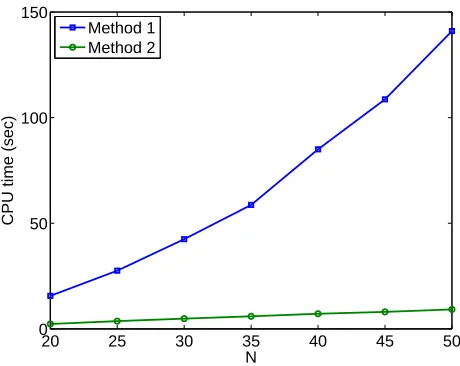
The Matlab routinefminconwas used to preform the resulting optimization problems for 100 independent simulated data sets. We considered 2 methods for computing the gradients. For method 1, we computed the gradient using a forward difference of the objective function J(α, µ). This method is equivalent to the default method for computing the gradient if the
user does not supply the gradient to fmincon. For method 2 we computed the gradient according to (2.13)−(2.15). In Figure 1 we depict the average cpu time required to complete the optimization using both methods for 100 independent data sets as N, the number of elements in the approximation scheme, increases.
Using method 1 requires N2 +N(κ+ 1) evaluations of v(x, t;θ, µ), whereas method 2
20 25 30 35 40 45 50 0
50 100 150
N
CPU time (sec)
Method 1 Method 2
Figure 1: The average cpu time (for 100 independent data sets) required to complete the optimization as N increases using both methods.
4
Example: Reflectance spectroscopy model
Here we describe an example from [5] where the model is an aggregate model. In this project, the goal is to develop a noninvasive technique to characterize the degradation of a complex nonmagnetic dielectric material by assessing the small physical and chemical changes in the material using reflectance spectroscopy. This involves determining the components of the permittivity of the dielectric medium using the measured spectral responses. The distributed relative permittivity of the dielectric medium is described by
b
εr(k;G,q) =ε∞−
Z
Ω
k2 p
k2 −ik/τ−k2 0
dG(k0). (4.1)
In the above equation, ε∞ denotes the relative permittivity of the dielectric medium at
infinite frequency, k is the wavenumber (k = ω/(2πc), where ω is the angular frequency and c is the speed of light), k0 represents the resonance wavenumbers, and τ denotes the
relaxation time. The composite parameterkp is given bykp =k0√εs−ε∞with εs being the
relative permittivity of the medium at zero frequency, i =√−1 is the imaginary unit, and θ =k0 ∈Ω⊂R. If we assume that a monochromatic uniform wave is incident at an angle of
φ = 45◦ on a plane interface between free space and a nonmagnetic dielectric medium with
the electric field composed of the parallel and perpendicular polarizations in equal weights, then the reflection coefficient is given by
R(k;G,q) = 1
2 |r⊥(k;G,q)|
2+
|rk(k;G,q)|2
, (4.2)
where
r⊥(k;G,q) =
cosφ−pεbr(k;G,q)−sinφ
cosφ+pbεr(k;G,q)−sinφ
, (4.3)
and
rk(k;G,q) =
p
1−sin2φ/εbr(k;G,q)−
p b
εr(k;G,q) cosφ
p
1−sin2φ/
b
εr(k;G,q) +
p b
εr(k;G,q) cosφ
In this application, the reflectance R(k;G,q) is measured at various wave numbers k in order to determine the distribution G(θ) =G(k0) of resonance wave numbers as well as
the parameters q= [εs, ε∞, τ]T. Data sets which were collected using a Bruker Vertex 80V
FTIR spectrometer have been provided by researchers at the Air Force Research Lab at Wright-Patterson Air Force Base. For a full description of the model, data collection, and subsequent inverse problems, see [5].
In this case the spline approximation scheme was used to estimate the probability measure G(θ), thus the permittivity model can be written as
b
εr(k;G,q) =ε∞−
N
X
m=1
αm
Z
Ωm
θ2(ε
s−ε∞)
k2−ik/τ −θ2lm(θ)dθ. (4.5)
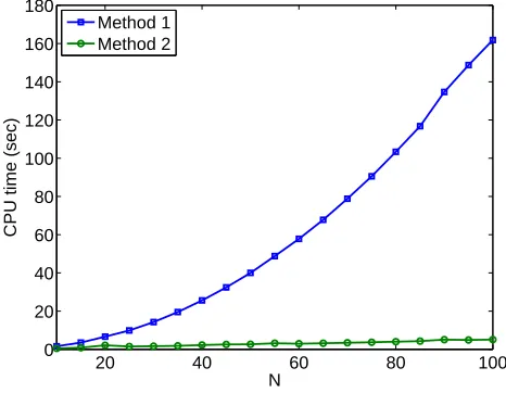
Again we use two methods to compute the gradient ofJ(α,q), where method 1 computes the gradient according to (2.9) and method 2 employs (2.13) where the integral terms in (4.5) were computed only once. In Figure 2 we show the average over 100 trials of the cpu time required to preform the first 10 iterations of the optimization problems as N is increased. As expected, we see that method 1 increases quadratically and method 2 linearly.
20 40 60 80 100
0 20 40 60 80 100 120 140 160 180
N
CPU time (sec)
Method 1 Method 2
Figure 2: The average cpu time (for 100 independent data sets) required to compute the first 10 iterations of the optimization problems as N increases using both methods.
5
Conclusions
In this paper we consider the case of non-parametric estimation of a probability measure under the Prohorov Metric Framework in a least squares problem. It is demonstrated that the gradient computation can be reduced by exploiting the linearity of the coefficients to be estimated which appear in the approximation schemes under the PMF.
For individual models the number of forward solves of the underlying model v is reduced fromO(N2) toO(N), where N is the number of elements in the approximation. Due to the
model with aggregate data is discussed and the expected linear increase in cpu time as N increases was observed.
For aggregate models the reduction of computational expense in computing the gradient of the objective function is not as straight forward. This is due directly to the fact that the model depends explicitly on the probability measure for aggregate models. However, we still can reduce the number of evaluations of the kernel functionf in (2.17) fromO(N2) toO(N).
The practical degree to which any speed up can be obtained in the inverse problem depends directly on the complexity of the kernel functionf. Iff is relatively cheap to evaluate, then the speed up may be negligible, even though we have reduced the number of evaluations. However, if f is costly to evaluate, then the speed up may be significant. We demonstrated this in an example arising in an application using reflectance spectroscopy, and the cpu time was observed to have the expected linear behavior.
Acknowledgments
This research was supported in part by the Air Force Office of Scientific Research under grant number AFOSR FA9550-12-1-0188, and in part by the US Department of Education Grad-uate Assistance in Areas of National Need (GAANN) under grant number P200A120047.
References
[1] H.T. Banks, A Functional Analysis Framework for Modeling, Estimation and Control in Science and Engineering, Chapman and Hall/CRC Press, Boca Raton, FL, 2012.
[2] H.T. Banks, L.W. Botsford, F. Kappel, and C. Wang, Modeling and estimation in size structured population models, LCDS-CCS Report 87-13, Brown University; Proceed-ings 2nd Course on Mathematical Ecology, (Triests, December 8-12, 1986) World Press (1988), Singapore, 521–541.
[3] H.T. Banks and D.M. Bortz, Inverse problems for a class of measure dependent dynam-ical systems, J. Inverse and Ill-posed Problems, 13 (2005), 103–121.
[4] H.T. Banks, D.M. Bortz and S.E. Holte, Incorporation of variability into the mathe-matical modeling of viral delays in HIV infection dynamics, Mathematical Biosciences,
83 (2003), 63–91.
[5] H.T. Banks, J. Catenacci and A. Criner, Quantifying the degradation in thermally treated ceramic matrix composite, CRSC-TR15-10, September, 2015; International J. Applied Electromagnetics (submitted).
[7] H.T. Banks and N.L. Gibson, Well-posedness in Maxwell systems with distributions of polarization relaxation parameters, CRSC-TR04-01, January, 2004; Applied Math. Letters,18 (2005), 423–430.
[8] H.T. Banks and N.L. Gibson, Electromagnetic inverse problems involving distributions of dielectric mechanisms and parameters, CRSC-TR05-29, August 2005; Quarterly of Applied Mathematics,64 (2006), 749–795.
[9] H.T. Banks, S. Hu, Z.R. Kenz, C. Kruse, S. Shaw, J.R. Whiteman, M.P. Brewin, S.E. Greenwald and M.J. Birch, Material parameter estimation and hypothesis testing on a 1D viscoelastic stenosis model: methodology, CRSC-TR12-09, April, 2012; J. Inverse and Ill-posed Problems, 21 (2013), 25–57.
[10] H.T. Banks and G.A. Pinter, A probabilistic multi scale approach to hysteresis in shear wave propagation in biotissue, CRSC-TR04-03, January, 2004;SIAM J. Multiscale Mod-eling and Simulation, 3(2005), 395–412.
[11] H. T. Banks, S. Hu, and W. C. Thompson, Modeling and Inverse Problems in the Presence of Uncertainty, CRSC Press/ Taylor & Frances Publishing, Boca Raton, FL, 2014.
[12] Lee J. Byrne, Diana J. Cole, Brian S. Cox, Martin S. Ridout, Byron J. T. Morgan, and Mick F. Tuite, The number and transmission of [PSI+] prion seeds (Propagons) in the
yeast Saccharomyces cerevisiae, PLoS ONE, 4(3) (2009), e4670.
[13] Brian Cox, Frederique Ness and Mick Tuite, Analysis of the generation and segretation of Propagons: Entities that propagate the [PSI+] prion in yeast, Genetics, 165 (2003),
23–33.
[14] Christopher J. Doona, Florence E. Feeherry, and Edward W. Ross, A quasi-chemical model for the growth and death of microorganisms in foods by non-thermal and high-pressure processing, Int. J. Food Microbiol., 100 (2005), 21–32.
[15] C. T. Kelley, Iterative Methods for Optimization, SIAM, Philadelpha, PA, 1999.
[16] Peter Olofsson and Suzanne S. Sindi, A Crump-Mode-Jagers branching process model of prion loss in yeast, J. Appl. Prob., 51 (2014), 453–465.
[17] K.J. Palmer, M.S. Ridout, and B.J.T. Morgan, Kinetic models of guanidine hydrochloride-induced curing of the yeast [PSI+] prion, J. Theoretical Biology, 274
(2011), 1–11.
[18] E.W. Ross, I.A. Taub, C.J. Doona, F.E. Feeherry, and K. Kustin, The mathematical properties of the quasi-chemical model for microorganism growth-death kinetics in foods,
Int. J. Food Microbiol., 99 (2005), 157–171.
[19] S.I. Rubinow, Introduction to Mathematical Biology, John Wiley & Sons, New York, NY, 1975.
[21] Lee A. Segel, Modeling Dynamic Phenomena in Molecular and Cellular Biology, Cam-bridge University Press, CamCam-bridge, UK, 1984
[22] Vinicio Serment-Moreno, Gustavo Barbosa-Canovas, Jose Antonio Torres, and Jorge Welti-Chanes, High-pressure processing: Kinetic models for microbial and enzyme in-activation, Food Eng. Rev., 6 (2014), 56–88.