ABSTRACT
LAW, SHIRLEY ELIZABETH. Combinatorial Realization of Certain Hopf Algebras of Pattern-Avoiding Permutations. (Under the direction of Nathan Reading.)
A general lattice theoretic construction of Reading constructs Hopf subalgebras of the
Malvenuto-Reutenauer Hopf algebra (MR) of permutations. The products and coproducts of
these Hopf subalgebras are defined extrinsically in terms of the embedding in MR. This thesis
further develops the understanding of these Hopf subalgebras. The goal is to find an intrinsic
combinatorial description of a particular family of these Hopf subalgebras. A simple Hopf
alge-bra in the family has a natural basis given by permutations that we call Pell permutations. The
Pell permutations are in bijection with combinatorial objects that we call sashes, that is, tilings
of a 1 by n rectangle with three types of tiles: black 1 by 1 squares, white 1 by 1 squares, and
white 1 by 2 rectangles. The bijection induces a Hopf algebra structure on sashes. We describe
the product and coproduct in terms of sashes, and the natural partial order on sashes. We also
describe the dual coproduct and dual product of the dual Hopf algebra of sashes. In general, this
family of Hopf subalgebras has a natural basis that is in bijection with combinatorial objects
that we call partial evaluations. We give a description of the product and the partial order of
©Copyright 2013 by Shirley Elizabeth Law
Combinatorial Realization of Certain Hopf Algebras of Pattern-Avoiding Permutations
by
Shirley Elizabeth Law
A dissertation submitted to the Graduate Faculty of North Carolina State University
in partial fulfillment of the requirements for the Degree of
Doctor of Philosophy
Mathematics
Raleigh, North Carolina
2013
APPROVED BY:
Patricia Hersh Tom Lada
DEDICATION
A.M.D.G.
BIOGRAPHY
Shirley Elizabeth Law was raised in Chapel Hill, North Carolina and graduated from East
Chapel Hill High School in 2003. She developed an interest in math from an early age by
working logic puzzles with her father. Shirley attended college at Appalachian State University.
In 2007 she received a Bachelor of Science in Mathematics, a Bachelor of Arts in Economics,
and a minor in Statistics. She continued her studies at North Carolina State University where
she received a Master of Science in Mathematics in 2009. From 2009 to 2010, Shirley lived and
worked at a university in Henan, China teaching Finance and English. She returned to North
Carolina State University to complete a Doctor of Philosophy in Mathematics. Her field of
ACKNOWLEDGEMENTS
Dr. Nathan Reading, my advisor, has taught me more than I could have imagined about math,
combinatorics, academia, and most importantly about life. I am tremendously grateful for the
countless hours he has spent helping me with all kinds of problems, and I particularly appreciate
his innumerable corrections. Nathan has provided me with many opportunities such as summer
research and international conference travel, for which I am much obliged. I could not have
asked for a better advisor. I am more and more appreciative of being able to work with Nathan
every day. Nathan is a man of high character and an excellent role model.
My parents, Gwillim and Janice Law, also deserve much acknowledgement. All of my
ac-complishments are founded on their undeserved love and support. I have always been able to
turn to them with any and every need, and they have been there for me every step of the way. I
am particularly grateful for all of the work my dad did editing this dissertation. His corrections
were very helpful.
Thank you to Drs. Jeffand Holly Hirst and Drs. Rick and Vicky Klima, my college professors,
for giving me confidence and for caring about me beyond the classroom.
I really appreciate Mrs. Sara Hinsley who put up with my shenanigans in high school, and
inspired me to pursue my interests in mathematics.
The Bible study of mathematics graduate students has been an invaluable source of prayers
and friendship. This group has helped me through the many difficulties of graduate school.
It has truly been a blessing to me. All of the members have been an encouragement to me,
but I would like to name a few by name: Alyssa Armstrong, Erin Bancroft, Eric Bancroft, Jeb
Collins, Sharon Moore, Erick Smith, Anastasia Wilson, and Cory Winton.
I would like to thank Dr. Vic Reiner for taking an interest in my work and for asking some
very insightful questions.
I would also like to acknowledge the NSF for support during the summer of 2012 under the
TABLE OF CONTENTS
LIST OF FIGURES . . . vi
Chapter 1 Introduction . . . 1
1.1 Background . . . 1
1.2 Hopf Algebra of Pattern-avoiding Permutations . . . 9
1.3 Combinatorial Realizations . . . 17
Chapter 2 The Hopf Algebra of Sashes . . . 19
2.1 Pell Permutations and Sashes . . . 19
2.2 The Hopf Algebra (and Dual Hopf Algebra) of Sashes . . . 24
2.2.1 Product . . . 25
2.2.2 Dual Coproduct . . . 26
2.2.3 Dual Product . . . 27
2.2.4 Coproduct . . . 30
Chapter 3 The Hopf Algebra of Partial Evaluations . . . 50
3.1 Limited Descent Avoiders and Partial Evaluations . . . 50
3.2 The Hopf Algebra of Partial Evaluations . . . 65
LIST OF FIGURES
Figure 1.1 Algebra Commutative Diagrams . . . 1
Figure 1.2 Coalgebra Commutative Diagrams . . . 2
Figure 1.3 Bialgebra Commutative Diagram . . . 2
Figure 1.4 Elements of Υnfor −1≤n≤3 . . . 5
Figure 1.5 The five planar binary trees in PBT3. . . 5
Figure 1.6 A diagonal rectangulation of size 20 . . . 6
Figure 1.7 A product calculation in the Hopf algebra dRec . . . 6
Figure 1.8 A product calculation in the Hopf algebra dRec . . . 7
Figure 1.9 A coproduct calculation in the Hopf algebra dRec . . . 8
Figure 2.1 The elements of Σ3 and Σ4. . . 20
Figure 2.2 The allowable dottings of a sash . . . 31
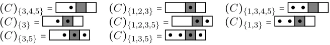
Figure 2.3 The allowable sets and allowable dottings of a sash C . . . 40
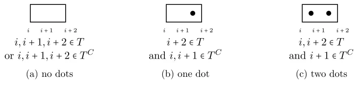
Figure 2.4 Possible rectangle dottings of the ith and(i+1)st positions ofC . . . . . 41
Figure 3.1 The fourteen partial evaluations of length 3, i.e.the elements of Σ3 . . . 54
Figure 3.2 A summary of black positions and white positions . . . 61
Chapter 1
Introduction
1.1
Background
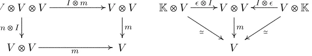
A unital associativealgebra over a fieldKis a vector spaceV overKwith an associative bilinear product m∶V ⊗V →V and a unit "∶K→V such that the diagrams in Figure 1.1 commute.
The map I is the identity from V to V. Similarly, a counital coassociative coalgebra over K is a vector spaceV over Kwith a coproduct∆∶V →V ⊗V and a counitζ ∶V →Ksuch that the
diagrams in Figure 1.2 commute.
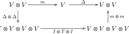
A bialgebra is a vector space that is both a unital associative algebra and a counital coasso-ciative coalgebra, such that the diagram in Figure 1.3 commutes. The mapT ∶V ⊗V →V ⊗V
is the twist map that sendsv2⊗v1↦v1⊗v2, for allv1, v2∈V. A graded vector space over Kis a direct sum ⊕
n≥0
Vn where each Vn is a finite dimensional
V ⊗V ⊗V
V ⊗V
V ⊗V
V ... . . . .
I⊗m
. . . . . . . . . . . . . . . . . . . . . . . . . . . . . . . . . . . . . . . . . . . . . . . . . . . . . . . . . . . . . . . . . . . ...
m⊗I
. ... . . . . m . . . . . . . . . . . . . . . . . . . . . . . . . . . . . . . . . . . . . . . . . . . . . . . . . . . . . . . . . . . . . . . . . . . . ... m
K⊗V V ⊗V V ⊗K
V . ... . . . .
!⊗I
. . . . . . . . . . . . . . . . . . . . . . . . . . . . . . . . . . . . . . . . . . . . . . . . . . . . . . . . . . . . . . . . . . ... ...
I⊗!
...≃... ... . . . . . . . . . . . . . . . . . . . . . . . . . . . . . . . . . . . . . . . . . . . . . . . . . . . . . . . . . . . . . . . . . . . . ... m . . . . . . . . . . . . . . . . . . . . . . . . . . . . . . . . . . . . . . . . . . . . . . . . . . . . . . . . . . . . . . . . . . . . . . . . . . . . . . . . . . . . . . . . . . . . . . . . . . . . . . . . . ... ... ≃
V
V ⊗V
V ⊗V
V ⊗V ⊗V
. ...∆... . . . . . . . . . . . . . . . . . . . . . . . . . . . . . . . . . . . . . . . . . . . . . . . . . . . . . . . . . . . . . . . . . . . . . ... ∆ ... . . .
I⊗∆
. . . . . . . . . . . . . . . . . . . . . . . . . . . . . . . . . . . . . . . . . . . . . . . . . . . . . . . . . . . . . . . . . . . ...
∆⊗I
K⊗V V ⊗V V ⊗K
V . . . . . . . . . . . . . . . . . . . . . . . . . . . . . . . . . . . . . . . . . . . . . . . . . . . . . . . . . . . . . . . . . . ... . ...
ζ⊗I
... . . . .
I⊗ζ
...≃... ... . . . . . . . . . . . . . . . . . . . . . . . . . . . . . . . . . . . . . . . . . . . . . . . . . . . . . . . . ... . . . . . . . . . . . . ∆ . . . . . . . . . . . . . . . . . . . . . . . . . . . . . . . . . . . . . . . . . . . . . . . . . . . . . . . . . . . . . . . . . . . . . . . . . . . . . . . . . . . . . . . . . . . . . . . . . . . . . . . . . ... ... ≃
Figure 1.2: Coalgebra Commutative Diagrams
V ⊗V
V ⊗V ⊗V ⊗V
V ⊗V
V ⊗V ⊗V ⊗V V
...m... . ...∆... . . . . . . . . . . . . . . . . . . . . . . . . . . . . . . . . . . . . . . . . . . . . . . . . . . . . . . . . . . . . . . . . . . . . ... ∆⊗∆ ... . . .
I⊗T⊗I
. . . . . . . . . . . . . . . . . . . . . . . . . . . . . . . . . . . . . . . . . . . . . . . . . . . . . . . . ... . . . . . . . . . . . .
m⊗m
Figure 1.3: Bialgebra Commutative Diagram
vector space overK. A bialgebra on a graded vector space V =⊕ n≥0
Vn is agraded bialgebra if m maps Vp⊗Vq to Vp+q for all p≥0 and q≥0, and if∆ mapsVn to ⊕
p+q=n
Vp⊗Vq.
In general, a Hopf algebra is a bialgebra, with an additional map from V to V called the
antipode, satisfying certain conditions. However, every graded bialgebra possesses an antipode. Thus a graded Hopf algebra is nothing more than a graded bialgebra. We refer to each graded
Hopf algebra by a triple(V, m,∆), whereV is a graded vector space, mis a product map, and
∆ is a coproduct map. More information about Hopf algebras (graded or not) can be found
in [14].
Example 1.1.1. LetV be a graded vector space of polynomials such that for each graden≥0,
the basis vector isxn. We will describe the Hopf algebra of polynomials by defining a product and a coproduct on the basis vectors.
m(xp⊗xq)=xp+q
∆(xn)= n
∑
i=0
The focus of this research is on combinatorial Hopf algebras: Hopf algebras such that the
basis elements of the underlying vector space are indexed by a family of combinatorial objects.
For eachn≥0, letOnbe a finite set of “combinatorial objects”. We define a graded vector space
over a field K, such that for each graden the basis vectors of the vector space are indexed by
the elements of On. That is, the graded vector space is: K[O∞]=⊕n≥0K[On]. For simplicity, we refer to a basis element of this vector space by the combinatorial object indexing it. There is
a more sophisticated approach for defining combinatorial Hopf algebras. For more information
see [1].
The Malvenuto-Reutenauer Hopf algebra of permutations (MR) is a graded combinatorial
Hopf Algebra (K[S∞],●,∆). Given a field K, let K[Sn] be a vector space whose basis
ele-ments are indexed by the eleele-ments of Sn, where Sn is the group of permutations of the set
[n]={1,2, . . . , n}. We identify the basis elements with the permutations themselves and thus write elements ofK[Sn] asK-linear combinations of permutations inSn.
The product in MR is called the shifted shuffle. To multiply two permutations,
x = x1x2⋯xp ∈ Sp and y = y1y2⋯yq ∈ Sq, we begin by shifting y. Define y′ = y′1⋯y′q where y′
i =yi+p. A shifted shuffle of x and y is a permutation z∈Sn where n=p+q, such that the total order of the entries 1 through pofz, is given byx, and the total order of the entriesp+1
through n of z, is given by y′. The product of x and y in MR is the sum of all the shifted
shuffles of xand y and is denoted by either m(x⊗y) or x●y.
Example 1.1.2. The product of two basis elements 21 and 312:
21●312= 21534+25134+25314+25341+52134+
52314+52341+53214+53241+53421
The coproduct map is defined by separating a permutation in all possible places and then
standardizing the result. The notion of standardization is illustrated as part of Example 1.1.3, and a precise definition of standardization is given in Section 1.2. We standardize so that all
permutation 32154 between the 2 and the 1 we have 32 and 154. Standardizing these pieces
gives the term 21⊗132.
The coproduct in MR is
∆(x)= n ∑ i=0
st(x1⋯xi)⊗st(xi+1⋯xn)
where st(x1⋯x0)and st(xn+1⋯xn)are both interpreted as the empty permutation∅, the unique
element ofS0.
Example 1.1.3.
∆(32154)=∅ ⊗32154+1⊗2143+21⊗132+321⊗21+3214⊗1+32154⊗ ∅
Notice that the product is the sum of the natural ways of combining two basis elements,
and the coproduct is the sum of the natural ways of splitting a basis element into two pieces.
Another well-known combinatorial Hopf algebra is NSym [6]. NSym can be represented as
the Hopf algebra of noncommutative symmetric functions, the Hopf algebra of compositions, or
as the Hopf algebra of subsets, but we will describe it here in terms of another combinatorial
object: a tiling of a 1×n rectangle with black 1×1 squares and/or white 1×1 squares. This
representation will be relevant to the description of the Hopf algebra of Sashes in Chapter 2 and
to the description of the Hopf algebra of partial evaluations in Chapter 3. More information
about this Hopf algebra can be found in [2].
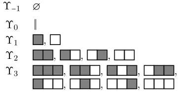
Fix a 1×nrectangle, and letΥnbe the set of tilings of that rectangle by black and/or white 1×1 squares, see Figure 1.4. We now describe the Hopf algebra(K[Υ∞],●Υ,∆Υ), whereK[Υ∞]=
⊕n≥0K[Υn−1]. Let A∈Υp and B ∈Υq. The product map is given by:A●ΥB=A B+A B. The coproduct is more complicated, so we will leave the description until Chapter 3.
An important Hopf subalgebra of MR is the Loday-Ronco Hopf algebra, defined on a graded
Υ−1 ∅
Υ0 ‖
Υ1 ,
Υ2 , , ,
Υ3 , , , ,
, , ,
Figure 1.4: Elements ofΥn for−1≤n≤3
Figure 1.5: The five planar binary trees in PBT3.
children or has two children, one designated as a right child and one as a left child. Vertices with no children are called leaves. We draw the trees with the leaves lined up horizontally and the root above them, with edges drawn so that, for each leaf, the path from that leaf to the
root is monotone up. Let PBTnbe the set of planar binary trees withn+1 leaves. For example,
the five trees of PBT3 are shown in Figure 1.5. A description of the product and coproduct of
this combinatorial graded Hopf algebra is found in [9].
The final combinatorial Hopf algebra we mention here is the Hopf algebra of diagonal
rect-angulations (K[dRec∞],●dR,∆dR) as described in [8]. A diagonal rectangulation of size n is a n×n square divided into n rectangles such that the interior of each rectangle intersects the
diagonal of the square with negative slope. The bottom left corner of the square is on the origin
of the Cartesian plane, and all points of intersection within the rectangulation have integer
coordinates. Figure 1.6 shows a diagonal rectangulation of size 20. The diagonal is shown in
gray. The number of diagonal rectangulations of sizen are counted by the Baxter numbers.
Let dRecnstand for the set of rectangulations of sizen. The set dRec0 has a single element,
repre-Figure 1.6: A diagonal rectangulation of size 20
●dR =sum of completions of
= + + + +
Figure 1.7: A product calculation in the Hopf algebra dRec
sented by the symbol∅. The set dRec1 also has a single element, the “division” of a square into
a single square. The Hopf algebra dRec is the graded vector spaceK[dRec∞]=⊕n≥0K[dRecn], with the product and coproduct that we now describe.
Let R1 ∈dRecp and R2 ∈dRecq, where p+q =n. The product in dRec is the sum over all
completions of the following “incomplete rectangulation”: An×nsquare with the interior ofR1 in the upper left corner and the interior of R2 in the lower right corner. That is, we sum over
all rectangulations of size n that can be defined by adding additional lines to the incomplete
rectangulation. We give two examples in Figures 1.7 and 1.8, marking, for the sake of clarity,
the point(p, n−p)in each diagonal rectangulation in the product.
Before we describe the coproduct ∆dR, we first need to define some terminology. Let R be a diagonal rectangulation of size n and consider any path γ from the top-left corner of R
to the bottom-right corner of R, traveling only along edges of rectangles, and traveling only
●dR =sum of completions of
= + + + + + .
Figure 1.8: A product calculation in the Hopf algebra dRec
p rectangles below/left of the path andq rectangles above/right of the path, with p+q=n.
We associate to the path γ an element Aγ⊗Bγ of dRec⊗dRec. If p=0 then the element
Aγ is ∅. Otherwise, Aγ is obtained as follows: First, delete from R everything that lies on
or is above/right of γ, except for the outer edges of the square. Then, scale this incomplete
rectangulation down to a p×p size square. The element Aγ is the sum over all completions of
this incomplete diagonal rectangulation. Similarly,Bγ=∅ifq=0, and otherwiseBγ is obtained
by deleting from R everything that lays on or is below/left ofγ, except for the outer edges of
the square, scaling the result to aq×q square, and then summing over all completions of the
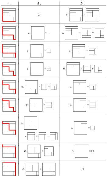
resulting incomplete diagonal rectangulation. The coproduct ofR is the sum, over all pathsγ,
of Aγ⊗Bγ.
Consider, for example, the coproduct of
.
Figure 1.9 shows each path γ and the associated Aγ and Bγ. The figure uses the abbreviation
γ Aγ Bγ
∅ c. =
c. = c. = +
c. = c. =
c. = c. = +
c. = + c. =
c. = c. =
c.
= + +
c. =
c. = c. =
c. = ∅
1.2
Hopf Algebra of Pattern-avoiding Permutations
Let Sn be the group of permutations of the set [n] = {1,2, . . . , n}. Also define [n, n′] = {n, n+1, . . . , n′} for n′ ≥ n. For x =x1x2⋯xn ∈Sn, an inversion of x is a pair (xi, xj) where
i<j and xi >xj, and the inversion set of x is the set of all such inversions. The weak order is the partial order on Sn with x ≤x′ if and only if the inversion set of x is contained in the inversion set of x′. The weak order is a lattice. The inverse x−1 of a permutationx∈S
n is the permutation x−1=y=y
1⋯yn∈Sn such thatyi =j whenxj=i.
Let T be a set consisting of integers t1 < t2 < ⋯ < tn. Given a permutation x ∈ Sn, the notation(x)T stands for the permutation ofT whose one-line notation hastj in theithposition when xi=j. On the other hand, given a permutationx of T, thestandardization, st(x), is the unique permutation y∈Sn such that(y)T =x.
Now let T be a subset of [n]. For x ∈ Sn, the permutation x∣T is the permutation of T obtained by removing from the one-line notation forx all entries that are not elements of T.
Example 1.2.1. Let x=31254, T1={2,3,6,8,9}, andT2={2,3,5}. Then,(x)T1 =62398 and
thus st(62398)=31254. Also, x∣T2 =325.
The Malvenuto-Reutenauer Hopf algebra MR is a graded Hopf Algebra(K[S∞],●,∆), as we
explained in Section 1.1. We now reiterate a description of MR with more detail and with some
variations to notation. LetK[S∞]=⊕n≥0K[Sn]be a graded vector space. Letx=x1x2⋯xp∈Sp andy=y1y2⋯yq∈Sq. Definey′=y′1⋯y′qto be(y)[p+1,p+q] so thaty′i=yi+p. Ashifted shuffle of x and y′ is a permutation z∈Sn where n=p+q,z∣[p]=x and z∣[p+1,n]=y′. The product of x
and y in MR is the sum of all the shifted shuffles of x and y. Equivalently,
x●y=∑[x⋅y′, y′⋅x] (1.1)
sum of all the elements in the weak order interval[x⋅y′, y′⋅x]. The coproduct in MR is:
∆(x)= p ∑ i=0
st(x1⋯xi)⊗st(xi+1⋯xp) (1.2)
where st(x1⋯x0) and st(xp+1⋯xp) are both interpreted as the empty permutation∅.
Define the map Inv ∶ Sn → Sn by Inv(x) = x−1 and extend the map linearly to a map
Inv ∶ KS∞ → KS∞. MR is known to be self dual [10] and specifically Inv is an isomorphism
from (K[S∞],●,∆) to the graded dual Hopf algebra (K[S∞],∆∗, m∗). Let x ∈Sp,y∈Sq, and
z∈Sn, where p+q=n. Given a subsetT of p elements of [n],TC denotes the complement of T in[n]. The dual product is given by:
∆∗(x⊗y)=Inv(x−1●y−1)= ∑ T⊆[n],
∣T∣=p
(x)T ⋅(y)TC, (1.3)
and the dual coproduct is:
m∗(z)=(Inv⊗Inv)(∆(z−1))= n ∑ i=0
z∣[i]⊗st(z∣[i+1,n]) (1.4)
wherez∣[0] and z∣[n+1,n] are both interpreted as the empty permutation ∅.
Now that we have explicitly described both the Hopf algebra of permutations and the dual
Hopf algebra of permutations, we will present a family of Hopf subalgebras that are defined by a
particular pattern-avoidance condition. This family of Hopf algebras is defined by Reading [12].
For some k ≥ 2, let V ⊆ [2, k−1] such that ∣V∣ = j and let VC be the complement of V in [2, k−1]. A permutation x ∈ Sn avoids the pattern V(k1)VC if for every subsequence xi1xi2⋯xik of x with ij+2 = ij+1 +1, the standardization st(xi1xi2⋯xik) is not of the form
v(k1)v′ for any permutation v of the set V and any permutation v′ of VC. In the notation of Babson and Steingrimsson [4] avoiding V(k1)VC means avoiding all patterns of the form v1−⋯−vj−k1−v1′−⋯−v′
k−j−2, wherev1⋯vj is a permutation ofV andv
′
Let U be a set of patterns of the form V(k1)VC, where ∣V∣ and k can vary. Define Avn to be the set of permutations in Sn that avoid all of the patterns in U. We define a graded
Hopf algebra(K[Av∞],●Av,∆Av)as a graded Hopf subalgebra of MR. LetK[Avn]be a vector
space, over a field K, with basis vectors indexed by the elements of Avn, and let K[Av∞] be
the graded vector space ⊕n≥0K[Avn]. The product and coproduct on K[Av∞] are described
below.
We define a map π↓∶Sn→Avn recursively. If x∈Avn then define π↓(x)=x. If x∈Sn, but x ∉Avn, then x contains an instance of a pattern V(k1)VC in U. That is, there exists some subsequencexi1xi2⋯xik of x, whereij+2=ij+1+1 andj=∣V∣, such thatst(xi1xi2⋯xik)=vk1v
′
for some permutations v and v′ of V and VC. Exchange xij+1 and xij+2 in x to create a new permutation x′, calculate π↓(x′) recursively and setπ↓(x)=π↓(x′). The recursion must
termi-nate because an inversion ofx is destroyed at every step, and because the identity permutation
is in Avn. The map π↓is well-defined as explained in [12, Remark 9.5]. We emphasize that the
definition ofπ↓is dependent on U.
The map π↓ defines an equivalence relation with permutations x, x′ ∈Sn equivalent if and only if π↓(x)=π↓(x′). The set Avn is a set of representatives of these equivalence classes. This equivalence relation is a lattice congruence on the weak order. Therefore the poset induced
on Avn by the weak order is a lattice (also denoted by Avn) and the map π↓ is a lattice
homomorphism from the weak order to Avn. The congruence classes defined byπ↓are intervals,
andπ↓maps an element to the minimal element of its congruence class. Letπ↑be the map that
takes an element to the maximal element of its congruence class.
The following proposition is a special case of [12, Proposition 2.2]. The congruence on Sn defined byπ↓ is denoted byΘ. Forx∈Sn, the congruence class of xmod Θis denoted by [x]Θ.
Proposition 1.2.2. Given Sn a finite lattice, Θ a congruence on Sn, and x ∈ Sn, the map
y→[y]Θ restricts to a one-to-one correspondence between elements ofSn covered by π↓(x) and
Example 1.2.3. A well known lattice is the Tamari lattice which is isomorphic to Avn for
U = {2(31)}. Let Gn be the set of objects of this lattice. The elements of Gn are strings of
n factors grouped into pairs by n−1 sets of parentheses. The partial order relation for the
Tamari lattice is (A(BC)) Ì((AB)C), where A, B, and C are elements of Gh, Gi, and Gj respectively, for some 1≤h, i, j≤n−2 such thath+i+j=n.
Both π↓ and π↑ are order preserving and π↑○π↓ = π↑ and π↓○π↑ = π↓. A π↓-move is the
result of switching two adjacent entries of a permutation in the manner described above. That
is, it changes⋯k1⋯to ⋯1k⋯for some pattern in U. A π↑-move is the result of switching two
adjacent entries of a permutation in a way such that a π↑-move undoes aπ
↓-move. That is, it
changes⋯1k⋯to ⋯k1⋯.
We define a map r ∶K[S∞] → K[Av∞] that identifies the representative of a congruence
class. Givenx∈Sn,
r(x)=⎧⎪⎪⎪⎪⎪⎨ ⎪⎪⎪⎪⎪ ⎩
x if x∈Avn
0 otherwise.
Similarly, we define a map c ∶ K[Av∞] → K[S∞] that takes an avoider to the sum of its
congruence class:
c(x)= ∑ ysuch that
π↓(y)=x y.
We now describe the product and coproduct in (K[Av∞],●Av,∆Av). Let x∈Avp, and let y∈Avq. Then:
mAv(x⊗y)=x●Avy=r(x●y). (1.5)
Just as the product in MR is ∑[x⋅y′, y′⋅x], we can view this product as:
x●Avy=∑[x⋅y′,π↓(y′⋅x)], (1.6)
The coproduct is:
∆Av(z)=(r⊗r)(∆(c(z))). (1.7)
We now describe the Hopf algebra (K[Av∞],∆∗Av,●∗Av)that is dual to(K[Av∞],●Av,∆Av).
We extend the map π↓ linearly, soπ↓ is a map from K[S∞] to K[Av∞]. The map that is dual
to the map c is c∗ ∶K[S
∞]→K[Av∞], where c∗(x) =π↓(x) for x ∈ K[S∞]. The map that is
dual to the map r is r∗∶K[Av∞]→K[S∞], wherer∗(x)=x forx∈K[Av∞].
Let z ∈Avn, where n=p+q. The dual coproduct is given by dualizing Equation (1.5), so
that:
m∗Av(z)=m∗(z). (1.8)
The dual product ∆∗
Av is given by dualizing Equation (1.7):
∆∗Av(x⊗y)=π↓∆∗(x⊗y). (1.9)
Combining Equation (1.9) with Equation (1.3), we have:
∆∗Av(x⊗y)= ∑ T⊆[n]
∣T∣=p
π↓((x)T ⋅(y)TC) (1.10)
Equation (1.10) leads to the following order theoretic description of the coproduct ∆Av,
which was worked out jointly with Nathan Reading.
Given z ∈ Avn, a subset T ⊆ [n] is good with respect to z if there exists a permutation z′=z′
1⋯zn′ withπ↓(z′)=z such thatT={z1′, . . . , z∣′T∣}. SupposeT is good with respect to z, let
p=∣T∣ and let q =n−p. Let zmin be minimal, in the weak order on Sn, among permutations equivalent to z and whose firstp entries are the elements of T. Let zmax be maximal, in the
weak order, among such permutations. DefineIT to be the sum over the elements in the interval
Theorem 1.2.4. Let z∈Avn. Then
∆Av(z)= ∑
T is good
IT ⊗JT
where IT =∑[st(zmin∣T),π↓st(zmax∣T)], JT =∑[st(zmin∣TC),π↓st(zmax∣TC)].
To prove Theorem 1.2.4, we first need several lemmas.
Lemma 1.2.5. The elements in the interval [zmin, zmax] are equivalent to z and their first p
entries are the elements of T.
Proof. All of the elements in the interval [zmin, zmax] are equivalent to z because equivalence classes are intervals in the weak order. To prove the rest of the lemma, suppose for the sake of
contradiction that there is an elementz′∈[z
min, zmax]whose firstpentries are not the elements of T. That is, z′ has some y ∈ TC before some x ∈ T. If x < y, then (y, x) ∈ Inv(z′), but
(y, x) ∉Inv(zmax), so z′ ∉ [zmin, zmax]. If y < x, then (x, y) ∈ Inv(zmin), but (x, y) ∉ Inv(z′), soz′∉[z
min, zmax]. Therefore the first p entries of elements in the interval [zmin, zmax] are the elements ofT.
Lemma 1.2.6. Suppose T ⊆ [n] with ∣T∣ = p. Let q = n−p. Suppose also that x1 ≤ x2 ≤ x3
in Avp, and that y1 ≤ y2 ≤ y3 in Avq. If π↓((x1)T ⋅(y1)TC) = π↓((x3)T ⋅(y3)TC) = z, then
π↓((x2)T ⋅(y2)TC)=z.
Proof. If x1 ≤x2 ≤x3, and y1 ≤y2 ≤y3, then (x1)T ⋅(y1)TC ≤(x2)T ⋅(y2)TC ≤(x3)T ⋅(y3)TC.
Sinceπ↓is an order preserving map,π↓((x1)T⋅(y1)TC)≤π↓((x2)T⋅(y2)TC)≤π↓((x3)T⋅(y3)TC).
The assertion of the lemma follows.
Lemma 1.2.7. Suppose x1, x2 ∈Sp and y1, y2∈Sq. Suppose T ⊆[n], where n=p+q, and with
∣T∣=p. The following identities hold:
(x1)T ⋅(y1)TC∨(x2)T ⋅(y2)TC =(x1∨x2)T ⋅(y1∨y2)TC
Proof. First we consider the identity with joins. There are three different kinds of inversions in (x1)T ⋅(y1)TC: inversions withinx1, inversions withiny1, and inversions betweenTandTC. The
inversion set of the permutation on the left hand side of the equation is the union of: inversions
withinx1in terms of T, inversions withiny1in terms of TC, inversions withinx2in terms of T, inversions withiny2 in terms of TC, and inversions betweenT and TC. Similarly, the inversion set of the permutation on the right hand side of the equation is the union of: inversions within
x1 or x2 in terms ofT, inversions withiny1 or y2 in terms ofTC, and inversions betweenT and TC. Therefore the permutation on the left hand of the equation and the permutation on the right hand of the equation have identical inversion sets and are thus the same.
The proof for the identity with meets is identical except for examining intersections of the
inversion sets instead of unions.
Proof of Theorem 1.2.4. In light of Equation (1.10), ∆Av(z) is the sum, overT ⊆[n], of terms x⊗y∈Avp⊗Avq such that π↓((x)T⋅(y)TC)=z. Some termsx⊗y may appear in∆Av(z)with coefficient greater than 1, but for each T, a term x⊗y occurs at most once. Let terms(z, T)
be the set {x⊗y ∶π↓((x)T ⋅(y)TC)=z}. It is immediate that when terms(z, T) is nonempty,
T is good with respect to z. On the other hand, if T is good with respect to z, then let z′
have π↓(z′)=z and {z1′, z2′, . . . , z∣′T∣}=T. Let x∈Sp and y ∈Sq be such that z
′=(x)
T ⋅(y)TC.
Then π↓(x)∈Avp and π↓(y)∈Avq. Since π↓(x) is obtained from x by a sequence ofπ↓-moves,
and π↓(y) is obtained similarly from y, we see that (π↓(x))T ⋅(π↓(y))TC is obtained from
z′ = (x)T ⋅(y)TC by a sequence of π↓-moves. Thus, π↓((π↓(x))T ⋅(π↓(y))TC) = π↓(z′) = z, so
π↓(x)⊗π↓(y)∈terms(z, t) and in particular terms(z, T) is nonempty.
Next, we need to show that, for each good subset T, the set terms(z, T) is of the form
IT ⊗JT. For convenience, we consider eachx⊗y as an element of Avp×Avq without rewriting
x⊗y as(x, y).
Suppose x1⊗y1 andx2⊗y2 are in terms(z, T). Then by Lemma 1.2.7,
Since π↓ is a lattice homomorphisim, the latter is
π↓((x1)T ⋅(y1)TC)∨π↓((x2)T ⋅(y2)TC)=z∨z=z.
Thus(x1∨x2)⊗(y1∨y2) is in terms(z, T). The same argument holds for meets, so terms(z, T)
is closed under meets and joins in the product order Avp×Avq. Lemma 1.2.6 implies that
terms(z, T) is order-convex in Avp×Avq. An order-convex subset that is closed under meets
and joins is necessarily an interval.
Suppose x⊗y < st(zmin∣T)⊗st(zmin∣TC) in Avp×Avq. Then (x)T ⋅(y)TC < zmin in Sn.
Thus π↓((x)T ⋅(y)TC)≠ z, by the definition of zmin, and therefore x⊗y ∈/terms(z, T). Thus
st(zmin∣T)⊗st(zmin∣TC) is the minimal element of terms(z, T).
Now suppose x⊗y > π↓st(zmax∣T)⊗π↓st(zmax∣TC) in Avp×Avq. Then since π↑ is
order-preserving andπ↑○π↓=π↑, we see thatπ↑(x)⊗π↑(y)>π↑st(zmax∣T)⊗π↑st(zmax∣TC). Thus on
the lattice Sn,
(π↑(x))T ⋅(π↑(y))TC >(π ↑
st(zmax∣T))T ⋅(π↑st(zmax∣TC))
TC. (1.11)
The right side of Equation (1.11) is obtained from zmax by standardizing the first part of the
permutation, doing someπ↑-moves, unstandardizing, and then repeating for the last part of the
permutation. The same result can be obtained by simply applying the correspondingπ↑-moves to
zmax, without standardizing and unstandardizing. In particular, the right side of Equation (1.11)
is greater than or equal to zmax. Now Equation (1.11) implies that (π↑(x))
T ⋅(π
↑(y))
TC is
strictly greater than zmax. The definition ofzmax says that π↑(x)⊗π↑(y)∈/terms(z, T). Thus (π↑(x))
T ⋅(π
↑(y))
TC is not equivalent to z.
But (π↑(x))T ⋅(π↑(y))TC is obtained from (x)T ⋅(y)TC by standardizing the first part,
doing some π↑-moves, unstandardizing, and then repeating for the last part. The same result
is again obtained by simply applying the the correspondingπ↑-moves to (x)T ⋅(y)TC, without
standardizing and unstandardizing. Thus (π↑(x))
T ⋅(π
↑(y))
which is therefore not equivalent to z. We have shown thatx⊗y/∈terms(z, T).
Thus, we have shown that terms(z, T) equals
[st(zmin∣T)⊗st(zmin∣TC),π↓st(zmax∣T)⊗π↓st(zmax∣TC)].
Any interval in Avp×Avq is the product of an interval in Avp with an interval in Avq. Thus
terms(z, T) is IT ⊗JT.
The proof of Theorem 1.2.4 also establishes the following more detailed statement.
Proposition 1.2.8. For some T ⊆ [n], x⊗y ∈ terms(z, T) if and only if x⊗y is a term of
IT ⊗JT in ∆Av(z).
Proof. Since x⊗y ∈terms(z, T) means thatπ↓((x)T ⋅(y)TC)=z, we see from Equation(1.10)
and Theorem 1.2.4 that for a fixed set T, x⊗y is a term of the summand indexed by T in
∆Av(z) if and only if z is the summand indexed byT in ∆∗Av(x⊗y).
1.3
Combinatorial Realizations
All of the Hopf algebras described in Section 1.1 are Hopf subalgebras of MR. Also, each is
isomorphic to (K[Av∞],●Av,∆Av) for choices of U shown here.
Object U
polynomial {(21)}
black/white square tilings {2(31),(31)2}
planar binary trees {2(31)}
diagonal rectangulations {2(41)3,3(41)2}
In Chapter 2, we consider a particular Hopf algebra given by U = {2(31),(41)23} and
describe it in terms of a natural combinatorial object. To begin, we compute how many basis
vectors the Hopf subalgebra has for each grade. Next we find a combinatorial object that
combinatorial objects by using the bijection to map the combinatorial objects to permutations,
computing the operation on the permutations, and then mapping the permutations back to the
combinatorial object. However, the goal of this research is to find an intrinsic representation of
these operations; an operation directly on the objects that will produce the same output as the
method described.
ForU ={2(31),(41)23}, the set Avnis counted by the Pell numbers, so(K[Av∞],●Av,∆Av)
might be called the Hopf algebra of Pell permutations. In Section 2.1 we define Pell
permu-tations, and we also introduce a combinatorial object called sashes. There is a bijection from
Pell permutations to sashes which is used to determine the operations on the Hopf algebra of
sashes.
In Section 2.2 we describe the Hopf algebra of sashes and the dual Hopf algebra of sashes
by defining the product, dual coproduct, dual product, and coproduct intrinsically. These four
operations are all defined directly in terms of sashes.
In Chapter 3, we consider a family of Hopf subalgebras of which the Hopf Algebra of
sashes is a member. This family is indexed by a parameter k, and each Hopf Algebra is
(K[Av∞],●Av,∆Av), for U ={2(31),(k1)23⋯k−1}. We realize these Hopf algebras via combi-natorial objects we call partial evaluations. In Section 3.1, we describe the avoiders Avn. Then we define a bijection from avoiders to partial evaluations. In Section 3.2 we describe the product
Chapter 2
The Hopf Algebra of Sashes
2.1
Pell Permutations and Sashes
In this section, we describe a particular combinatorial Hopf algebra that is isomorphic to a Hopf
subalgebra of pattern-avoiding permutations. To begin, we define a set of permutations called
Pell permutations.
Given a permutation x = x1x2⋯xn ∈ Sn, for each i ∈ [n−1], there is a nonzero integer j such thatxi=xi+1+j. Ifj>0, then there is andescent of sizej in theith position ofx. A Pell permutation is a permutation of [n] with no descents of size larger than 2, and such that for
each descent xi =xi+1+2, the element xi+1+1 is to the right of xi+1. We write Pn for the set of Pell permutations inSn.
Let us consider how many Pell permutations of length n there are. Givenx∈Pn−1, we can
place n at the end of x or before n−1. We can also place n beforen−2, but only if n−1 is
the last entry of x. Therefore ∣Pn∣=2∣Pn−1∣+∣Pn−2∣. This recursion, with the initial conditions ∣P0∣=0 and∣P1∣=1, defines the Pell numbers as defined by [13, Sequence A000129].
Lemma 2.1.1. Pn=Avn for U ={2(31),(41)23}.
(a)Σ3
(b)Σ4
Figure 2.1: The elements ofΣ3 andΣ4.
2(31). Now supposex∈Avn. Supposexhas a descentxi=xi+1+j. Becausex avoids 2(31), the entries xi+1+1, ..., xi+1+j−1 are to the right of the xi+1. Thus, since x avoids (41)23 we see thatj≤2 and conclude thatx∈Pn.
The poset induced on Pn by the weak order is a lattice (also denoted by Pn). As a conse-quence of Lemma 2.1.1, there is a Hopf algebra (K[Av∞],●Av,∆Av) of Pell permutations. For
the rest of this chapter we fix U ={2(31),(41)23}.
There is a combinatorial object in bijection with Pell permutations that will allow us to
have a more natural understanding of the Hopf algebra of Pell permutations.
A sash of lengthnis a tiling of a 1×nrectangle by black 1×1 squares, white 1×1 squares,
and/or white 1×2 rectangles. The set of sashes of lengthnis called Σn. There are no sashes of length -1 soΣ−1=∅, and there is one sash of length 0, a 1 by 0 rectangle denoted‖, so∣Σ0∣=1.
There are two sashes of length 1: and . The five sashes of length 2 and the twelve sashes
of length 3 are shown in Figure 2.1. The poset structure of these sashes will be explained later
in this section.
∣Σn∣=2∣Σn−1∣+∣Σn−2∣. Since∣Σ−1∣=0 and∣Σ0∣=1, there is a bijection between Pell permutations of lengthnand sashes of lengthn−1. We now describe a bijection that we use to induce a Hopf
Algebra structure on sashes.
Definition 2.1.2. We define a mapσ fromSn toΣn−1. Letx∈Sn. We build a sash σ(x) from
left to right as we consider the entries in x from 1 ton−1. For each value i∈[n−1], ifi+1 is
to the right of i, place a black square on the sash, and if i+1 is to the left of i, place a white
square on the sash. There is one exception: If i+1 is to the right of i, and i+2 is to the left
of i(and of i+1), then place a rectangle in the ith and (i+1)st positions of the sash. We also
defineσ(1)=‖and σ(∅)=∅.
From the definition of the map σ we see that σ sometimes involves replacing an adjacent
black square and white square by a rectangle. Later, we will sometimes break a rectangle into
a black square and a white square.
Example 2.1.3. Here is the procedure for computingσ(421365).
2 is to the left of 1 →
3 is to the right of 2 →
4 is to the left of 3 and also to the left of 2 →
5 is to the right of 4 →
6 is to the left of 5 but to the right of 4 →
Let T be a set of nintegers and let xbe a permutation ofT. We define σ(x)=σ(st(x)).
Example 2.1.4. σ(742598)=σ(st(742598)) =σ(421365)=
Definition 2.1.5. We define a map η∶Σn−1 →Pn. To calculate η(A) for a sash A∈Σn−1, we
place the numbers 1 throughn one at a time. Place the number 1 to begin and leti run from
1 ton−1. IfA has either a black square or the left half of a rectangle in theith position, place i+1 at the right end of the permutation. If A has either a white square or the right half of a rectangle in theith position, placei+1 immediately to the left ofiori−1 respectively. We also
It is immediate that this construction yields a Pell permutation because the output has no
descents of size larger than 2, and for each descent of size 2, the value in between the values of
the descent is to the right of the descent.
Example 2.1.6. Here are the steps to calculate η(A)for A= .
→ 1
→ 21
→ 213
→ 4213
→ 42135
→ 421365
Theorem 2.1.7. The restriction of σ to the Pell permutations is a bijection σ ∶Pn → Σn−1
whose inverse is given byη∶Σn−1→Pn.
Proof. Let A ∈Σn−1. We first show that σ(η(A)) =A. If A has a black square in position i, thenη(A) hasi+1 to the right of iand i+2 not to the left of i. So σ(η(A)) also has a black square in theith position. IfAhas a white square in positioni, thenη(A) hasi+1 immediately
to the left ofi. Soσ(η(A)) also has a white square in the ith position. If A has a rectangle in positionsiandi+1, thenη(A)hasi+1 to the right ofi, andi+2 immediately to the left ofi. So
σ(η(A)) also has a rectangle in theith and (i+1)stpositions. We conclude that σ(η(A))=A. We have constructed a Pell permutation η(A) that maps to A under σ, therefore σ is
surjective. Since we know∣Pn∣=∣Σn−1∣, the mapσ restricted to Pell permutations is a bijection. The inverse map of σ is η.
Proposition 2.1.8. x, y∈Sn are equivalent if and only ifσ(x)=σ(y).
Proof. The permutations x=x1⋯xn and y=y1⋯yn are equivalent if and only if π↓(x)=π↓(y).
Thus to prove the forward direction of the proposition, it is enough to consider the case wherey
σ, thusσ(x)=σ(y). Now we suppose thatxi=xi+1+2. There can only be aπ↓-move switching
xi and xi+1 of x if xi+1+1 is to the left of xi. In this case, both σ(x) and σ(y) have a white square in the ith position and a black square in the(i+1)st position. Thereforeσ(x)=σ(y).
To prove the reverse implication suppose that x and y are not equivalent, that is
π↓(x) ≠ π↓(y). Since π↓(x) and π↓(y) are Pell permutations, and σ is a bijection from Pell
permutations to sashes,σ(π↓(x))≠σ(π↓(y)). But by the previous paragraph, σ(π↓(x))=σ(x)
and σ(π↓(y))=σ(y).
The partial order onΣn−1 is such that the mapσ∶Pn→Σn−1 is an order isomorphism from the lattice of Pell permutations toΣn−1. We refer to this lattice as Σn−1.
From Proposition 1.2.2, the cover relations in Σn−1 are exactly the relations σ(y) Ìσ(x) wherex∈Pn and y is covered byx inSn.
Proposition 2.1.9. The cover relations on sashes are
1. A B ÌA B for any sash A and for a sash B whose leftmost tile is not a white square
2. A B ÌA B for any sashA and any sash B
3. A B ÌA B for any sashA and any sash B
Proof. Let x ∈ Pn and let y ∈ Sn such that y is covered by x in the weak order. That is, x=x1⋯xixi+1⋯xn and y=x1⋯xi+1xi⋯xn∈Snfor somexi>xi+1.
Suppose xi =xi+1+1 and xi+1 is not to the left of xi. Let A =σ(x∣[1,xi+1])=σ(y∣[1,xi+1]) and letB=σ(x∣[xi,n])=σ(y∣[xi,n]). Thus,A B=σ(y)Ìσ(x)=A B, where the leftmost tile of B is not a white square.
Suppose xi=xi+1+1 andxi+1 is to the left of xi. Let A=σ(x∣[1,xi+1])=σ(y∣[1,xi+1]) and let B=σ(x∣[xi+1,n])=σ(y∣[xi+1,n]). Thus,A B=σ(y)Ìσ(x)=A B.
Supposexi=xi+1+2. LetA=σ(x∣[1,xi+1])=σ(y∣[1,xi+1])and let B=σ(x∣[xi,n])=σ(y∣[xi,n]).
Thus,A B =σ(y)Ìσ(x)=A B.
2.2
The Hopf Algebra (and Dual Hopf Algebra) of Sashes
The bijection σ allows us to carry the Hopf algebra structure on Pell permutations to a Hopf
algebra structure (K[Σ∞],●S,∆S) on sashes and a dual Hopf algebra (K[Σ∞],∆∗S, m∗S) on
sashes, where K[Σ∞] is a vector space, over a field K, whose basis elements are indexed by
sashes. In order to do this, we extend σ and η to linear maps. For each grade nof the vector
space, the basis elements are represented by the sashes of length n−1. Recall that the sash of
length -1 is represented by∅, and the sash of length 0 is represented by‖. LetA,B, andC be
sashes. Using σ, we define a product, coproduct, dual product, and dual coproduct of sashes:
mS(A, B)=A●SB=σ(η(A)●Avη(B)) (2.1)
∆S(C)=(σ⊗σ)(∆Av(η(C))) (2.2)
∆∗
S(A⊗B)=σ(∆Av∗ (η(A)⊗η(B))) (2.3)
m∗S(C)=(σ⊗σ)(m∗Av(η(C))) (2.4)
These operation definitions are somewhat unsatisfying because they require computing the
operation in MR. That is, calculating a product or coproduct in this way requires mapping
sashes to permutations, performing the operations in MR, throwing out the non-avoiders in the
result, and then mapping the remaining permutations back to sashes. In the rest of this chapter
2.2.1 Product
Proposition 2.2.1. The empty sash∅is the identity for the product ●S. For sashes A≠∅ and
B≠∅, the product A●SB equals: ⎧⎪⎪⎪⎪ ⎪⎪ ⎨⎪⎪⎪ ⎪⎪⎪⎩
∑ [A B, A′ B] if A=A′
∑ [A B, A B] if A≠A′
where ∑[D, E] is the sum of all the sashes in the interval [D, E] on the lattice of sashes.
To clarify, here are some more specific cases of the product on sashes. If A = A′ , then
∑ [A B, A′ B]equals:
⎧⎪⎪⎪⎪ ⎪⎪ ⎨⎪⎪⎪ ⎪⎪⎪⎩
A B+A B′+A B+A′ B if B= B′
A B+A B+A′ B if B≠ B′
and if A≠A′ , then∑ [A B, A B]equals:
⎧⎪⎪⎪⎪ ⎪⎪ ⎨⎪⎪⎪ ⎪⎪⎪⎩
A B+A B′+A B if B= B′
A B+A B if B≠ B′
The case where A=‖is an instance of A≠A′ , and similarly for B=‖.
Proof. We begin by computing the product of Pell permutations. We showed in Section 1.2 that the product of Pell permutations is the sum over the interval[x⋅y′,π↓(y′⋅x)]in the lattice of
Pell permutations, where x∈Pp,y∈Pq, andy′=(y)[p+1,n].
To compute the product of sashes we can apply the map σ to the product of Pell
permu-tations. Let σ(x) = A and σ(y) = B, thus A●S B = σ(x●P y) = ∑[σ(x⋅y′),σ(π
↓(y′⋅x))] =
∑[σ(x⋅y′),σ(y′⋅x)]. The mapσ takes the firstp values of x⋅y′ to A and the lastq values to
Similarly,σ takes the firstp values ofy′⋅x toA and the lastq values toB. Sincep+1 is to the
left ofp, to computeσ(y′⋅x)we need to consider whether or notp−1 is beforep inx.
Supposep−1 is beforepinx. Thus,Aends with a black square soσ(y′⋅x) replaces the last
black square ofA with a rectangle in positions p−1 and p. That is σ(y′⋅x)=A′ B, where
A=A′ .
Suppose p−1 is not before p inx. Thus, A either ends with a white square, the right half
of a rectangle, orp−1 does not exist. Thus,σ(y′⋅x)places a white square after Aand before
B, soσ(y′⋅x)=A B.
In informal terms, the product of two sashes is the sum of the sashes created by joining the
two sashes with a black square and a white square, and if by so doing an adjacent black square
to the left of a white square is created, then the product has additional terms with rectangles
in the places of the adjacent black square and white square.
Example 2.2.2. Let A = and let B = . Notice that for A′ = and B′ =‖, both
A=A′ and B= B′.
A●SB= A B + A B′+ A B + A′ B
●S = + + +
2.2.2 Dual Coproduct
From Equation (1.8) and Equation (1.4), it follows that:
m∗S(C)= n ∑ i=0
σ(η(C)∣[i])⊗σ(η(C)∣[i+1,n]) (2.5)
Proposition 2.2.3. The dual coproduct on a sash C∈Σn is given by:
m∗S(C)= n ∑ i=−1
Ci⊗Cn−i−1
in which case Ci ends with ), and Cn−i−1 ∈ Σn−i−1 is a sash identical to the last n−i−1 positions of C (unless C has in position i+2, in which case Cn−i−1 begins with ), and we define C0 =C0=‖ and C−1=C−1=∅.
Proof. We need to show that C is a term of A●SB if and only if A⊗B is a term of m∗S(C). Suppose that C∈Σn is a term ofA●SB, withA∈Σp,B∈Σq, and p+q=n−1. ThusC is one of the following:A B,A B,A′ B, orA B′, forA′and B′as in Proposition 2.2.1.
In any case, m∗
S(C) has a term A⊗B becauseCp=A and Cn−p−1=B.
Now suppose that for A∈ Σp and B ∈Σq, A⊗B is a term of m∗S(C), where C ∈ Σn and p+q = n−1. Thus Cp = A and Cn−p−1 = Cq = B. If C is A B or A B, then C is a term of A●SB. If C is A′ B, then A=A′ , and C is a term of A●
SB. If C is A B′, then B= B′, and C is a term of A●
SB. Therefore in all cases C is a term of A●SB and we have shown that the map m∗
S is the dual coproduct on sashes.
2.2.3 Dual Product
From Equation (1.9), it follows that:
∆∗S(A⊗B)= ∑ T⊆[n]
∣T∣=p
σ((η(A))T ⋅(η(B))TC) (2.6)
We now prepare to describe the dual product ∆∗
S directly on sashes.
Definition 2.2.4. Given a setT ⊆[n]such that∣T∣=pandn=p+q, and given sashesD∈Σp−1
and E ∈Σq−1, define a sashγT(D⊗E) by the following steps. First, write D above E. Then,
label D with T, by placing the elements of T in increasing order between each position of D,
Example 2.2.5. LetT ={1,2,4,7,8,9,12,13}, D= , and E=
1 2 4 7 8 9 12 13
3 5 6 10 11 14 15
Next, draw arrows from i to i+1 for all i∈ [n−1]. Lastly, follow the path of the arrows
placing elements in a new sash based on the following criteria:
Place a rectangle in the ith and (i+1)st positions of the new sash if either of the following
conditions are met:
1. if the ith arrow is from D to E, the (i+1)st arrow is from E to D, and there is a or inDin betweeniand i+2
2. if theith arrow is fromE toE, the (i+1)starrow is fromE toD, and there is a or inE in between iand i+1
If the above criteria are not met, then the following rules apply:
1. if theith arrow is fromDtoD(or from E toE), place whatever is in between iandi+1
inD(or in E) in theith position.
2. if theith arrow is fromDto E, place a black square in theith position.
3. if theith arrow is fromE to D, place a white square in theith position.
Note that it may be necessary to replace the left half of a rectangle by a black square or
to replace the right half of a rectangle by a white square (as in the first step of the example
Example 2.2.6. Let T, D, and E be as in Example 2.2.5. Then we compute γT(D⊗E) to
obtain:γ{1,2,4,7,8,9,12,13}( ⊗ )= .
1 2 4 7 8 9 12 13
3 5 6 10 11 14 15 !
" " "#$$
$$% " " "# ! ""
""&
! ! ' ' ' (! $$
$$% !
' ' '
(! 2⇒
Theorem 2.2.7. The dual product of sashes D∈Σp−1 and E∈Σq−1, for p+q=n, is given by:
∆∗S(D⊗E)= ∑ T⊆[n],
∣T∣=p
γT(D⊗E)
Proof. For D∈Σp−1 and E ∈Σq−1 such that η(D)=x∈Pp and η(E)=y∈Pq, where p+q=n, we consider Equation (2.6) to define the dual product of sashes.
Let T ⊆[n] such that∣T∣=p. It is just left to show thatγT(D⊗E)=σ((x)T ⋅(y)TC).
Case 1: i, i+2∈T andi+1∈TC such thati+2 is to the left ofi in(x)T.
γT(D⊗E) outputs a rectangle in the ith and (i+1)st positions because theith arrow is from D to E, the(i+1)st arrow is fromE to D, and there is a or inD in between the labels iand i+2. The sashσ((x)T ⋅(y)TC) has a rectangle in the ith and (i+1)st positions because
i+1 is to the right ofi, and becausei+2 is to the left of i.
Case 2: i, i+1∈TC and i+2∈T such thati+1 is to the right ofi in(y)TC.
γT(D⊗E) outputs a rectangle in the ith and (i+1)st positions because theith arrow is from E to E, the (i+1)st arrow is from E to D, and there is a or in E in between the labels iand i+1. The sashσ((x)T ⋅(y)TC) has a rectangle in the ith and (i+1)st positions because
i+1 is to the right ofi, and becausei+2 is to the left of i.
Case 3: i∈T,i+1∈TC, and if i+2∈T, theni+2 is to the right of iin(x)T.
ith position because i+1 is to the right ofi, and becausei+2 is not to the left of i.
Case 4:i∈TC,i+1∈T, ifi−1∈T theni+1 is to the right ofi−1 in(x)T, and ifi−1∈TC
theniis to the left of i−1 in (y)TC.
γT(D⊗E)outputs a white square in the ith position because theith arrow is fromE toD, and the criteria to place a rectangle is not met. The sashσ((x)T ⋅(y)TC)has a white square in the
ith position because i+1 is to the left ofi, and becausei−1 is not in between i+1 andi.
Case 5: i, i+1∈T.
γT(D⊗E) outputs whatever is in between the labels iand i+1 inD in the ith position. The sash σ((x)T ⋅(y)TC) has the same.
Case 6: i, i+1∈TC, and if i+2∈T then i+1 is to the left of iin(y)TC.
γT(D⊗E) outputs whatever is in between the labels iand i+1 in E in theith position. The
sash σ((x)T ⋅(y)TC) has the same.
Therefore we have shown thatσ((x)T⋅(y)TC)andγT(D⊗E)have the same object in every
position.
2.2.4 Coproduct
We now describe the coproduct in the Hopf algebra of sashes and we begin with some definitions.
Definition 2.2.8. For C ∈ Σn−1, a dotting of C is C with a dot in any subset of the n−1
positions of C. An allowable dotting of C is a dotting of C that meets all of the following conditions
1. has at least one dot
2. the first dot can be in any position, and dotted positions alternate between a black square
(or the left half of a rectangle) and a white square (or the right half of a rectangle)
Figure 2.2: The allowable dottings of a sash
Figure 2.2 shows the allowable dottings of the sash .
Consider an allowable dotting d=c1●1c2●2⋯cj●jcj+1 of a sash C, where each ci is a sub sash ofC without any dots, and●i is a single dotted position. If any●i is on the right half of a
rectangle, then the the left half of the rectangle in the last position ofci is replaced by a black square. If ●i and ●i+1 are in adjacent positions, then ci+1 =‖. (If any●i is on the left half of a rectangle, then ●i+1 is on the right half of the same rectangle, so ci+1=‖.)
We use C and d to define two objects A and B that are similar to sashes, but have an
additional type of square , which we call a mystery square. If ●1 is on a black square or the
left half of a rectangle, then letA be the concatenation of the odd ci with a mystery square in between eachci (where iis odd), and letB be the concatenation of theeven ci with a mystery square in between each ci (where i is even). For example, if ●1 is on a black square and j is even, then A=c1 c3 ⋯ cj+1 and B =c2 c4 ⋯ cj. If●1 is on a white square or the right half of a rectangle, then let Abe the concatenation of the even ci with a mystery square in between each ci, and letB be the concatenation of theodd ci with a mystery square in between each ci.
We use the objects A and B to define four sashes A,A,B, and B.
To computeA, consider each mystery square inA. If the mystery square follows ci and the
ithand(i+1)stdots ofdare on the same rectangle, , then replace the mystery square after ci with a white square. Otherwise replace the mystery square with a black square.
To compute A, consider each mystery square in A from left to right. If the mystery square
If the mystery square is followed by a white square (i.e. if ci+2 starts with a white square),
then replace the mystery square and the white square with a rectangle. Otherwise replace the
mystery square with a black square. If the mystery square follows ci and the ith and (i+1)st
dots of darenot on an adjacent black square and white square, then we check to see whether or not the mystery square is preceded by a black square. If either ci ends in a black square or ci = ‖and the previous mystery square has been changed to a black square, then replace the mystery square afterci and the black square before it with a rectangle. Otherwise replace the mystery square after ci with a white square.
To compute B, replace all mystery squares ofB with black squares.
To compute B, replace all mystery squares of B with white squares, unless the mystery
square is preceded by a black square, in which case replace both the black square and the
mystery square with a rectangle.
Example 2.2.9. If d = , then c1 = , c2 = c3 = ,
c4 =c5 = c6 = ‖, c7 = , c8 = , c9 = c10 =c11 = ‖, and ●1 is on a black square. Thus,
A=c1 c3 c5 c7 c9 c11 and B=c2 c4 c6 c8 c10. Using the rules above
to computeA,B, and the four sashesA,A,B, and B, we have:
A= B=
A= B=
A= B=
Given an allowable dotting d of a sash C we define Id=∑ [A, A]and Jd=∑ [B, B] forA, A,B, and B computed as above. Thus the notation Id⊗Jd denotes∑D∈[A,A]
E∈[B,B]
D⊗E.
Theorem 2.2.10. GivenC∈Σn−1:
∆S(C)=∅ ⊗C+C⊗ ∅+ ∑
allowable dottings
dofC
To prove Theorem 2.2.10, we need to introduce some more terminology. Given an allowable
dottingdof a sashCand the objectsAandBdefined above, we define two more objects ˆAand
ˆ
B. These objects are similar to sashes, but have three additional types of squares: , , and
. We call these squares: black-plus square, white-plus square, and mystery square respectively.
If ●i and ●i+1 are on an adjacent black square and white square,i.e. , then replace the
after ci on A with a on ˆA. If ●i and ●i+1 are on a rectangle, i.e. , then replace the after ci on A with a on ˆA. The resulting objects are ˆAand ˆB. NoteB=B.ˆ
We say that a sashDis of the form ˆAifDis identical to ˆAexcept for the following allowable
substitutions:
• A black-plus square on ˆA is replaced by a black square onD. • A white-plus square on ˆA is replaced by a white square on D.
• A mystery square on ˆA is replaced by a either a black square or a white square onD. • A black-plus square or a mystery square on ˆA, and a white square, a white-plus square,
or a mystery square following it, are replaced by a rectangle onD.
• A white-plus square or a mystery square on ˆA, and a black square, a black-plus square, or a mystery square preceding it, are replaced by a rectangle onD.
Similarly, a sash E is of the form ˆB if it follows the same rules as above. Since ˆB does not
have any black-plus squares or white-plus squares, E is of the form ˆB if E is identical to ˆB
except for the following allowable substitutions:
• A mystery square on ˆB is replaced by a either a black square or a white square onE. • A mystery square on ˆB, and a white square or a mystery square following it, are replaced
by a rectangle onE.
Lemma 2.2.11. The sash A is minimal with respect to sashes of the form A.ˆ
Proof. The sash A is of the form ˆA, because every white-plus square on ˆA is replaced by a white square on Aand every black-plus square and mystery square on ˆA is replaced by a black
square onA.
Suppose the sash A′ is obtained from A by going down by a cover relation. We want to
show that A′ is not of the form ˆA.
Case 1: A′=A
1 A2 and A=A1 A2, where the leftmost tile ofA2 is not a white square.
Let∣A1∣=i−1, soA′ has a black square in theith position andA has a white square in theith position. Thus, ˆA either has a white square or a white-plus square in the ith position. Either way,A′ is not of the form ˆA.
Case 2: A′=A
1 A2 and A=A1 A2.
Let ∣A1∣= i−1, so A′ has a black square and white square in the ith and (i+1)st positions and A has a rectangle in theith and (i+1)st positions. Thus, ˆAhas a rectangle in the ith and (i+1)st positions, and A′ is not of the form ˆA.
Case 3: A′=A1 A2 and A=A1 A2.
Let∣A1∣=i−1, soA′ has a rectangle in theithand (i+1)st positions andA has a white square in both the ith and (i+1)stpositions. There are four possibilities of what occupies the ith and (i+1)st positions of ˆA: , , , or . In any case,A′ is not of the form ˆA.
Lemma 2.2.12. The sash A is maximal with respect to sashes of the form A.ˆ
Proof. The sash Ais of the form ˆA, because black-plus squares followed by white-plus squares, mystery squares, or white squares on ˆA are replaced by a rectangle onA, white-plus squares
and mystery squares preceded by black-plus squares or black squares on ˆA are replaced by a
rectangle on A, all other black-plus squares on ˆA are replaced by black squares on A, and all
other white-plus squares and mystery squares on ˆA are replaced by white squares onA.
Suppose the sash A′ is obtained from A by going up by a cover relation. We want to show
Case 1: A=A1 A2 and A′=A1 A2, where the leftmost tile ofA2 is not a white square.
Let ∣A1∣=i−1, so A has a black square in the ith position and A′ has a white square in the ithposition. Thus, ˆAeither has a black square or a black-plus square in the ith position. Either way,A′ is not of the form ˆA.
Case 2: A=A1 A2 and A′=A1 A2.
Let∣A1∣=i−1, soAhas a black square and white square in theithand(i+1)stpositions andA′ has a rectangle in the ith and (i+1)st positions. Thus, ˆA has a black square and white square in theith and (i+1)st positions, andA′ is not of the form ˆA.
Case 3: A=A1 A2 and A′=A1 A2.
Let∣A1∣=i−1, soAhas a rectangle in theith and(i+1)st positions andA′ has a white square in both theith and (i+1)st positions. There are five possibilities of what occupies the ith and
(i+1)stpositions of ˆA: , , , , or . In any case,A′ is not of the form ˆA.
Lemma 2.2.13. The sash B is minimal with respect to sashes of the form B.ˆ
Proof. The sashB is of the form ˆB, because every mystery square on ˆB is replaced by a black square onB.
Suppose the sash B′ is obtained from B by going down by a cover relation. We want to
show that B′ is not of the form ˆB.
Case 1: B′=B1 B2 and B=B1 B2, where the leftmost tile of B2 is not a white square.
Let∣B1∣=i−1, soB′has a black square in the ithposition and B has a white square in the ith
position. Thus, ˆB has a white square in theith position, and B′ is not of the form ˆB.
Case 2: B′=B
1 B2 and B=B1 B2.
Let ∣B1∣= i−1, so B′ has a black square and white square in the ith and (i+1)st positions and B has a rectangle in theith and (i+1)st positions. Thus, ˆB has a rectangle in theith and (i+1)st positions, and B′ is not of the form ˆB.
Case 3: B′=B1 B2 and B=B1 B2.
in both the ith and (i+1)st positions. Thus, ˆB has a white square in both theith and(i+1)st
positions, andB′ is not of the form ˆB.
Lemma 2.2.14. The sash B is maximal with respect to sashes of the form Bˆ.
Proof. The sashB is of the form ˆB, because every mystery square on ˆB is replaced by a black square on B, unless it is preceded by a black square, in which case the black square and the
mystery square are replaced by a rectangle on B.
Suppose the sash B′ is obtained fromB by going up by a cover relation. We want to show
thatB′ is not of the form ˆB.
Case 1: B=B1 B2 andB′=B1 B2, where the leftmost tile of B2 is not a white square.
Let∣B1∣=i−1, soB has a black square in theith position andB′has a white square in the ith position. Thus, ˆB has a black square in theith position, andB′ is not of the form ˆB.
Case 2: B=B1 B2 and B′=B1 B2.
Let ∣B1∣ = i−1, so B has a black square and white square in the ith and (i+1)st positions and B′ has a rectangle in theith and(i+1)stpositions. Thus, ˆB has a black square and white square in the ith and(i+1)st positions, andB′ is not of the form ˆB.
Case 3: B=B1 B2 and B′=B1 B2.
Let∣B1∣=i−1, soB has a rectangle in theith and(i+1)stpositions andB′ has a white square in both the ith and (i+1)st positions. Thus, ˆB either has a rectangle or a black square and mystery square in theith and (i+1)st positions. Either way, B′ is not of the form ˆB.
Proposition 2.2.15. If a sash D is of the formA, thenˆ D∈[A, A].
Proof. Suppose that D is of the form ˆA and that D≠A. We want to show that there exists a sash D′ such thatD′ÌDand D′ is of the form ˆA.
Case 1: For some white-plus square of ˆA, it is not replaced by a white square onD.
Since D is of the form ˆA, the white-plus square of ˆA is preceded by either a black square, a
black-plus square, or a mystery square and is replaced by the right half of a rectangle on D.