Improved vertex chain code based mapping algorithm for curve length estimation

(1)

ISSN 1549-3636

Corresponding Author: Habibollah Haron, Faculty of Computer Science and Information Systems, University Technology Malaysia

Improved Vertex Chain Code Based Mapping

Algorithm for Curve Length Estimation

1

Habibollah Haron, 2Amjad Rehman, 1L.A. Wulandhari and 2Tanzila Saba

1

Faculty of Computer Science and Information Systems, University Technology,Malaysia

2

College of Computer and Information Sciences, Al-Imam M. Saud Islamic University Riyadh, KSA

Abstract: Problem statement: Image representation has always been an important and interesting topic in image processing and pattern recognition. However, curve tracing and its relative operations are the main bottleneck. Approach: This research presents the mapping algorithm that covers one of the vertex chain code cells, the rectangular-VCC cell. The mapping algorithm consists of a cell-representation algorithm that represents a thinned binary image in rectangular cells, a transcribing algorithm that transcribes the cells into vertex chain code and a validation algorithm that visualizes vertex chain code into rectangular cells. Results: The algorithms have been tested and validated by using three thinned binary images: L-block, hexagon and pentagon. Conclusion/Recommendations: The results show that this algorithm is capable of visualizing and transcribing them into vertex chain code.

Key word: Vertex Chain Code (VCC), Rectangular Cells, transcribing algorithms, Thinned Binary Image, validation algorithm, Freeman Chain Code (FCC), mapping algorithm, L-block hexagon, Pentagon, clockwise direction

INTRODUCTION

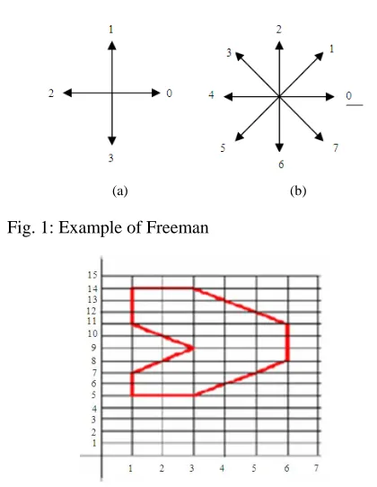
Image representation is an important component in image processing and pattern recognition. One of the ways to represent an image simply and efficiently is by using chain code. The first use of chain code was introduced by Freeman known as Freeman chain code (FCC). The code follows the contour counter-clockwise and keeps track of the direction from one contour pixel to the next (Saaid et al., 2009; Habibi et al., 2009; Jahanshah et al., 2009). The codes involve 4-connected and 8-connected paths. Figure 1(a) shows 4-connected and Fig. 1(b) shows 8-connected FCC

In the 8-connected FCC, each code can be considered as the angular direction, in multiples of 450, through which we must move to go from one contour pixel to the next. Figure 2 shows an example of Freeman Chain Code using an 8-connected path.

In general, a coding scheme for line structures must satisfy three objectives (Abdullah et al., 2009). First, it must faithfully preserve the information of interest; second, it must permit compact storage and be convenient for display. Finally, it must facilitate any required processing. The three objectives are somewhat in conflict with each other, and any code necessarily involves a compromise among them.

(a) (b)

Fig. 1: Example of Freeman

(2)

737

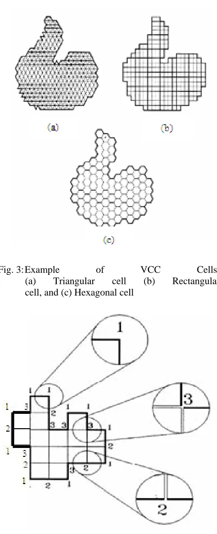
Fig. 3: Example of VCC Cells: (a) Triangular cell (b) Rectangular cell, and (c) Hexagonal cell

Fig. 4: The Example of Rectangular Cells-VCC VCC Code: 1233113121231212312131

Some important characteristic of the VCC as described in (Hashim and Marghany, 2009; Qicai et al., 2009; Al-Omari et al., 2009; Selvan et al., 2010) are first, the

VCC is invariant under translation and rotation, and optionally may be invariant under starting point and mirroring transformation. Second, using the VCC it is possible to represent shapes composed of triangular, rectangular, and hexagonal cells (Fig. 3). Thirdly, the chain elements represent real values not symbols such as other chain code; are part of the shape; indicate the number of cell vertices of the contour nodes; and may be operated for extracting interesting shape properties. Finally, using VCC it is possible to obtain relations between contours and the interior of the shape.

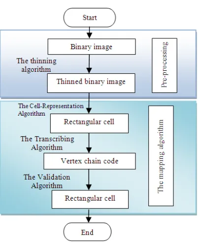
In the Vertex Chain Code, the boundaries or contours of any discrete shape composed of regular cells can be represented by chains. Therefore, these chains represent closed boundaries. The minimum perimeter of a closed boundary corresponds to the shape composed of only one cell. An element of a chain indicates the number of cell vertices, which are in touch with the bounding contour of the shape in that element position (Kumar et al., 2009). Figure 4 shows the Vertex chain code of Rectangular-VCC cells, indicating the number of cell vertices, in touch with the bounding contour of the rectangle in that element position.

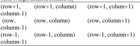
This paper presents an algorithms used to derive the rectangular cells of VCC from a thinned binary image, transcribed cells into vertex chain code and visualize the vertex chain code again into rectangular cells for validation. The algorithm is tested and validated using three thinned binary images: L-block, hexagon, and pentagon.

MATERIALS AND METHODS

(3)

Fig. 5: Flow of the mapping algorithm

Fig. 6: Binary image

Fig. 7: Thinned binary image

Pre-processing: This algorithm takes thinned binary image as input. Binary images have only two possible intensity values pixels and are normally displayed as black and white. Numerically, the two values are normally 0 for black and, either 1 or 255 for white. In the simplest case, an image may consist of a single object or several separated objects of relatively high intensity. In order to create the two-valued binary image, a simple threshold may be applied so that all the pixels in the image plane are classified into foreground (actual object) and background pixels. A binary image function can then be constructed such that pixels above the threshold are foreground (“1”) and below the threshold represent background (“0”) (Fig. 6).

For several purposes a binary image needs to be thinned. A thinned binary image is a binary image whose width is reduced to a single pixel (Fig. 7). The thinning process (Sikong et al., 2010) is an important pre-processing step in pattern analysis because it reduces memory requirements for storing the essential structural information presented in pattern. For this purpose, the thinning algorithm is created in (Marghany

et al., 2009) is applied. This thinning algorithm uses two-valued connectivity rules. The pixel of 1 will be replaced by pixel 0 when the number of pixels 1 of the neighbouring eight directions of connectivity pixel is greater than 3.

In this algorithm, every element of the thinned binary image is declared as an array variable. And all the operations of the images are according to rows and columns.

The mapping algorithm of rectangular-VCC: The Cell-representation Algorithm: The visualizing algorithm of Rectangular-VCC is an algorithm that represents a thinned binary image as rectangular cells. The algorithm has two-valued connectivity thinned binary images as input. Each code 1 in the thinned binary image represents each form of the rectangular cell. The direction of code 1 adjacent to another code 1 leads to the formation of the next rectangle. Figure 8 shows the representation of Rectangular-VCC formatted by the direction of code 1 adjacent to another code 1. When each code in the binary image is visualized, a line drawing consisting of rectangle cells will be created (Sarabian and Lee, 2010).

(4)

739

Fig. 1: Representation of rectangular-VCC

Table 1: Eight direction connectivity

(row+1, (row+1, column) (row+1, colum+1) column-1)

(row, (row, column) (row, column+1) column-1)

(row-1, (row-1, column) (row-1, column+1) column-1)

Based on these rules, the visualizing algorithm of rectangular VCC is created. The pseudo code of cell-presentation is presented in Appendix 1.

Appendix 1:

Input = thinned binary image image≠ 0

for row = 1 torow = maxrow

for column = 1 to column = maxcolum if image (row,column)= 1 then column _A = column+1 row_A = row +1 column_B = column -1 row_B = row – 1

if image (row, column_A) = 1 then for x = column to x<=column_A y = row

draw a horizontal line whose length = 1 from coordinate (x,y)

end for end if

if image (row_A, column)=1 then for y= row to y<=row_A x= column

draw a vertical line whose length = 1 from coordinate (x,y)

end for end if

if image (row_A, column_A)=1 then x = column_A

y = row_A

x = column y = row_A

end if

if image(row, column_B) = 1 then for x = column_B to x<= column y = row

end for end if

if image(row_A, column_B) = 1 then x = column

y = row

x = column_B y = row_A

end if

if image(row_B, column_B)=1 then x= column_B

y= row

x = column y = row

end if

if image(row_B,column) =1 then for y = row_B to y<=row x = column

end for end if

if image(baris_B, column_A) then x = column_A

y = row_B

x = column y = row

(5)

end for end for

Appendix 2:

Input = Rectangular-VCC and thinned binary image image

≠

0

for row = 1 torow = maxrow

for column = 1 to column = maxcolum if corner in position A then

if image (row,column)=1 and image (row,column_B)= 0 and image(row_B,column_B)=0 and image (row_B,column)=0 then VCC=1

end if

if image (row,column)=1 and image (row,column_B)= 1 and image(row_B,column_B)=0 and image (row_B,column)=0 then VCC = 2

end if

if image (row,column)=1 and image (row_B,column)= 1 and image(row,column_B)=0 and image (row_B,column_B)=0 then VCC = 2

end if

if image (row,column)=0 and image (row,column_B)= 1 and image(row_B,column)=1 and image (row_B,column_B)=0 then VCC = 3

end if end if

if corner in position B then

if image (row,column)=1 and image (row,column_A)= 0 and image(row_B,column)=0 and image (row_B,column_A)=0 then VCC=1

end if

if image (row,column)=1 and image (row,column_A)= 1 and image(row_B,column)=0 and image (row_B,column_A)=0 then VCC=2

end if

if image (row,column)=1 and image (row_B,column)= 1 and image(row,column_A)=0 and image (row_B,column_A)=0 then VCC=2

end if

if image (row,column)=0 and image (row,column_A)= 1 and image(row_B,column)=1 and image (row_B,column_A)=0 then VCC = 3

end if end if

if corner in position C then

if image (row,column)=1 and image (row_A,column)= 0 and image(row_A,column_A)=0 and image (row,column_A)=0 then VCC = 1

end if

if image (row,column)=1 and image (row_A,column)= 1 and image(row,column_A)=0 and image (row_A,column_A)=0 then VCC = 2

end if

if image (row,column)=1 and image (row,column_A)= 1 and image(row_A,column)=0 and image (row_A,column_A)=0 then VCC = 2

end if

if image (row,column)=0 and image (row_A,column)= 1 and image(row,column_A)=1 and image (row_A,column_A)=0 then VCC = 3

end if end if

if corner in position D then

if image (row,column)=1 and image (row_A,column_B)= 0 and image(row,column_B)=0 and image (row_A,column)=0 then VCC = 1

end if

if image (row,column)=1 and image (row_A,column)= 1 and image(row_A,column_B)=0 and image (row,column_B)=0 then VCC = 2

end if

if image (row,column)=1 and image (row,column_B)= 1 and image(row_A,column)=0 and image (row_A,column_B)=0 then VCC = 2

end if

if image (row,column)=0 and image (row_A,column)= 1 and image(row,column_B)=1 and image (row_A,column_B)=0 then VCC = 2

end if end if end for end for

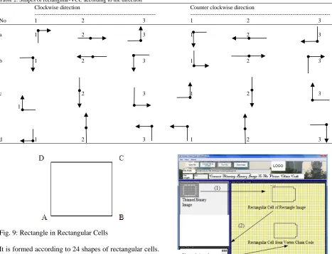
The transcribing algorithm: The transcribing algorithm converts the rectangular cells into vertex chain code. The algorithm uses 8-directions connectivity. Rectangular Vertex chain code has three different codes, namely 1, 2, and 3. The code indicates the number of cell vertices, which are in touch with the bounding contour of the shape in that element position. The algorithm focuses on the corner of each rectangular cell; the corners are named by A, B, C, and D (Fig. 9). The algorithm covers every corner of rectangle the by its own rules according to the eight-direction connectivity (Yang and Mareboyana, 2009). The algorithm that is to transcribe a thinned binary image into vertex chain code is shown in Appendix 2.

(6)

741 Table 2: Shapes of rectangular-VCC according to the direction

Clockwise direction Counter clockwise direction

--- ---

No 1 2 3 1 2 3

a 1 2 3 1 2 3

b 1 2 3 1 2 3

c 2 3 1 2 3

1

d 1 2 3 1 2 3

Fig. 9: Rectangle in Rectangular Cells

It is formed according to 24 shapes of rectangular cells. Every eight-shape represents every code 1, 2, and 3. Every code except the starting point code is used by previous code. This algorithm is invariant under the starting point, so it is immaterial which that is chosen as the starting point. Table 2 shows the shape of rectangular VCC according to direction (Yang and Mareboyana, 2009). Based on Table 2, the validation algorithm of rectangular VCC is created, also divided into two directions, because the difference in direction influences the next shape of the cells. Appendix 3 shows the validation algorithm of rectangular VCC.

RESULTS

All algorithms are tested and validated using three thinned binary images, L-block, hexagon, and pentagon. Thinned binary images are transformed into rectangular-VCC by using the cell-representation algorithm, rectangular-VCC is transcribed into Vertex Chain Cod using the transcribing algorithm, and finally Table 3 shows experimental results using the cell-representation, transcribing, and validation algorithms.

Fig. 10: The Interface of the Prototype System

The cell-representation and transcribing algorithms are validated by using the validation algorithm that visualizes the vertex chain code into rectangular cells again. The entire algorithm is termed as mapping algorithm.

The interface: The interface of the mapping algorithm of the rectangular VCC system is programmed in Visual Basic 6. Figure 10 shows the interface for testing and validating the mapping algorithm.

(7)

Table 3: Rectangular-VCC Cells and Vertex chain code of Three Thinned Binary Images (a) L-block, (b) Hexagon, (c) Pentagon

Rectangular VCC

No. Thinned Binary Image Rectangular VCC Cells Vertex chain code Cells (2)

a. 213131321321313131321313213131313

212131231313131313131213132131313231

313131231312313123131221313132131231

3131313131213131231

31313131313123131231313123131231

b. 22222222222222222213131313131313131312

1313131313131313131312222222222

222222221313131313131

31313121313131313131313131

c. 221321313132131321313132131313

12222222222222122222222222222

22222222212222222222222131

31312313131231312313131231

The interface shown in Fig. 10 consists of three processes involved in the mapping algorithm. The input is a thinned binary image. It is further represented as rectangular-VCC cells. The process continues by transcribing the rectangular-VCC cells into vertex chain code. The last process is to visualize the vertex chain code back into rectangular cells. The rectangular cell and code will be displayed automatically when the process is finished.

CONCLUSION

The mapping algorithm tested and validated in cell-representation and transcribing thinned binary images into VCC by using three thinned binary image objects, L-block, hexagon and pentagon. The results show that the cell-representation algorithm is capable of representing thinned binary image as rectangular-VCC cells. Reciprocally the transcribing algorithm is capable of transcribing the rectangular-VCC cells into vertex chain code and the validation algorithm result shows a rectangular cell that is similar with the rectangular cell from cell-representation algorithm. The entire algorithm is called the mapping algorithm of rectangular vertex chain code.

REFERENCES

Abdullah, H., A. Lennie, M.J. Saifuddin and I. Ahmad, 2009. The effect of electrical properties by texturing surface on gaas solar cell efficiency. Am. J. Eng. Applied Sci., 2: 189-193. DOI: 10.3844/ajeassp.2009.189.193

Al-Omari, S.A.K., P. Sumari, S.A. Al-Taweel and A.J.A. Husain, 2009. Digital recognition using neural network. J. Comput. Sci., 5: 427-434. DOI: 10.3844/jcssp.2009.427.434

Habibi, H. Shahmohammadi, V. Taraghi, S.D. Safari and B. Arezoo, 2009. A prototype two-axis laser scanning system used in stereolithography apparatus with new algorithms for computerized model slicing. Am. J. Applied Sci., 6: 1701-1707. DOI: 10.3844/ajassp.2009.1701.1707

Hashim, M. and M. Marghany, 2009. Robust of doppler centroid for mapping sea surface current by using radar satellite data. Am. J. Eng. Applied Sci., 2:781-788. DOI: 10.3844/ajeassp.2009.781.788 Jahanshah, F., K. Sopian, S.H. Zaidi, M.Y. Othman

and N. Amin et al., 2009. Modeling the effect of P-N junction depth on the output of planer and rectangular textured solar cells. Am. J. Applied Sci., 6: 667-671. DOI: 10.3844/ajassp.2009.667.671

Kumar, V.V., A. Srikrishna and G.H. Kumar, 2009. Error free iterative morphological decomposition algorithm for shape representation. J. Comput. Sci., 5: 71-78. DOI: 10.3844/jcssp.2009.71.78

Marghany, M., S. Mansor and M. Hashim, 2009. Geologic mapping of united Arab emirates using multispectral remotely sensed data. Am. J. Eng. Applied Sci., 2: 476-480. DOI: 10.3844/ajeassp.2009.476.480

Qicai, L., Z. Kai, Z. Zehao, F. Lengxi, O. Qishui and L. Xiu, 2009. The use of artificial neural networks in analysis cationic trypsinogen gene and hepatitis b surface antigen. Am. J. Immunol., 5: 50-55. DOI: 10.3844/ajisp.2009.50.55

(8)

743 Sarabian, M., and L.V. Lee, 2010. A modified partially

mapped multicrossover genetic algorithm for two-dimensional bin packing problem. J. Math. Stat., 6: 157-162. DOI: 10.3844/jmssp.2010.157.162 Selvan, S., M. Kavitha, S. Shenbagadevi and S. Suresh,

2010. Feature extraction for characterization of breast lesions in ultrasound echography and elastography. J. Comput. Sci., 6: 67-74. DOI: 10.3844/jcssp.2010.67.74

Sikong, L., B. Kongreong, D. Kantachote and W. Sutthisripok, 2010. Photocatalytic activity and antibacterial behavior of Fe3+-Doped TiO2/SnO2 nanoparticles. Energy Res. J., 1: 120-125. DOI: 10.3844/erjsp.2010.120.125