ABSTRACT
ZINK, JASON MICHAEL. Using Modern Photogrammetric Techniques to Map
Historical Shorelines and Analyze Shoreline Change Rates: Case Study on Bodie Island, North Carolina. (Under the direction of Dr. Margery F. Overton.)
The efficacy of coastal development regulations in North Carolina is dependent
on accurately calculated shoreline erosion rates. North Carolina’s current methodology
for regulatory erosion rate calculation does not take advantage of emerging GIS,
photogrammetric, and engineering technologies. Traditionally, historical shoreline
positions from a database created in the 1970s have been coupled with a modern
shoreline position to calculate erosion rates. The photos from which these historical
shorelines come were subject to errors of tilt, variable scale, lens distortion, and relief
displacement. Most of these errors could be removed using modern photogrammetric
methods. In this study, an effort was made to acquire and rectify, using digital image
processing, prints of the original historical photography for Bodie Island, North Carolina.
The photography was rectified using the latest available desktop photogrammetry
technology. Digitized shorelines were then compared to shorelines of similar date
created without the benefit of this modern technology. Uncertainty associated with
shoreline positions was documented throughout the process. It was found that the newly
created shorelines were significantly different than their counterparts created with analog
means. Many factors caused this difference, including: choice of basemaps, number of
tie points between photos, quality of ground control points, method of photo correction,
and shoreline delineation technique. Using both linear regression and the endpoint
method, a number of erosion rates were calculated with the available shorelines. Despite
rates were not significantly different. Specifically, the rate found using all available
shorelines prior to this study was very similar to the rate found using all shorelines
created in this study. As a result of this and other factors, it was concluded that a
complete reproduction of North Carolina’s historical shoreline database may not be
warranted. The new rectification procedure does have obvious value, and should be
utilized in those locations where there is no existing historical data, or where existing
data is thought to be of poor quality. This would especially be the case near inlets or
Using Modern Photogrammetric Techniques to Map Historical Shorelines and Analyze
Shoreline Change Rates: Case Study on Bodie Island, North Carolina
by
JASON MICHAEL ZINK
A thesis submitted to the Graduate Faculty of North Carolina State University
in partial fulfillment of the requirements for the Degree of
Master of Science
CIVIL ENGINEERING
Raleigh
2002
APPROVED BY:
___________________________________ ___________________________________
_________________________________
PERSONAL BIOGRAPHY
Jason Michael Zink was born in St. Louis, Missouri on October 3, 1978. He is the
only son of Michael and Sharon Zink of Huntersville, North Carolina and a brother to Alison.
Jason was a 1996 graduate of the North Carolina School of Science and Mathematics
(NCSSM) in Durham, North Carolina. He went on to attend the University of North
Carolina at Asheville where, in May 2000, he completed a B.A. in Mathematics. Time was
taken off both during and after undergraduate work to backpack the 2200 mile Appalachian
Trail, from Georgia to Maine. Jason began graduate work at North Carolina State University
in the spring of 2001 and has since pursued a Master of Science degree in Civil Engineering,
with a concentration in water resources and coastal engineering. As part of this degree
program, Jason has also completed a graduate minor in Geographic Information Systems
ACKNOWLEDGMENTS
The author would like to offer his sincere gratitude to Dr. Margery F. Overton and Dr.
John S. Fisher for their guidance and support throughout this research. Special thanks also
go to Stephen B. Benton of the Division of Coastal Management, who was able to provide
significant historical insight into erosion rate mapping procedures. Additional help in data
collection was provided by Dr. Robert Dolan of the University of Virginia, as well as Julia
Knisel at the Division of Coastal Management. Thanks to all previous and current students
involved in the NCSU Kenan Natural Hazards Mapping Program – including Melinda Koser,
Desiree Tullos, Rachel Smith, and Tiffany LaBrecque. Perhaps most importantly, the author
TABLE OF CONTENTS
Page
LIST OF TABLES vi
LIST OF FIGURES vii
LIST OF ABBREVIATIONS ix
1. INTRODUCTION 1
1.1. Use of Erosion Rates in Coastal Management Programs 1
1.2. Current Method of Calculating Rates in North Carolina 3
1.3. Research Objective 4
2. BACKGROUND 6
2.1. History of Aerial Photography 6
2.2. Sources of Error in Aerial Photography 7
2.3. Rectification Methods 11
3. STUDY AREA 14
3.1. Bodie Island, North Carolina 14
3.2. Storm History 16
4. DATA AND SOFTWARE 18
4.1. GIS and Image Processing Software 18
4.2. COAST Data Sets 19
4.3. T-sheet Data Sets 22
4.4. Newly Acquired Photography 25
5. METHODOLOGY 27
5.1. Image Processing 27
5.2. Shoreline Identification 37
6. ANALYSIS 42
6.1. Comparison of Shoreline Positions 43
6.2. Comparison of Methods 46
6.3. Comparison of Erosion Rates 52
7. RECOMMENDATIONS FOR FUTURE RESEARCH 64
8. SUMMARY AND CONCLUSIONS 66
9. REFERENCES 68
APPENDIX A. Coordinates and Descriptions of Ground Control Points
Used in Triangulation. 71
APPENDIX B. Images of Final Photo Mosaics for Seven Photo Dates. 75
APPENDIX C. Distances From Baseline for All Study Shorelines. 84
LIST OF TABLES
Page
Table 3-1. Pertinent storm events. 17
Table 4-1. Summary of shoreline data. 18
Table 4-2. Aerial photography acquired for rectification. 26
Table 5-1. Pixel size for scanned photos. 29
Table 5-2. Number of tie points per photo pair. 31
Table 6-1. Quantification of uncertainty for study shorelines. 43
Table 6-2. Positional comparison of COAST and new shorelines. 45
Table 6-3. Descriptions of calculated erosion rates. 52
Table 6-4. Summary of erosion rate comparisons. 63
Table A-1. Coordinates and descriptions of GCPs used in triangulation. 72
Table A-2. Distance between shorelines and baseline for study transects. 84
LIST OF FIGURES
Page
Figure 2-1. Effect of tilt on aerial photography. 9
Figure 3-1. Location maps: Bodie Island, North Carolina. 14
Figure 3-2. Oblique aerial photo of Bodie Island and Oregon Inlet,
April 6, 1999. 15
Figure 4-1. Basemaps HAT35, HAT36, HAT37, and HAT38 overlaid on the
COAST shoreline of December 13, 1962. 21
Figure 4-2. Scanned and digitized images of T-sheet T9278. 23
Figure 5-1. Flowchart of image processing procedures. 28
Figure 5-2. Point measurement window from ERDAS Imagine. 34
Figure 5-3. September 19, 1984 mosaic and close-up of photo intersection. 36
Figure 5-4. Digitized wet/dry line. 38
Figure 5-5. Intersection points of transects with baseline, December 1962 shoreline,
and June 1998 shoreline. 41
Figure 6-1. All COAST shorelines at intersection of basemaps HAT36 and HAT37. 44
Figure 6-2. USGS quad sheet with GCP from “old” rectification procedure. 49
Figure 6-3. Comparison of shoreline delineation methods. 51
Figure 6-4. Rates 3 and 4 for study transects. 53
Figure 6-5. Linear regression lines for rates 3 and 4 at transect 157. 54
Figure 6-6. Rates 5 and 6 for study transects. 55
Figure 6-7. Linear regression lines for Rates 5 and 6 at transect 157. 56
Figure 6-8. Rates 7 and 8 for study transects. 57
Figure 6-9. Rates 9 and 10 for study transects. 58
Figure 6-11. Rates 11 and 12 compared to Rates 9 and 10. 60
Figure 6-12. Rates 1, 2, 13, and 14 for study transects. 62
Figure A-1. Final mosaic and GCPs for March 14, 1962. 76
Figure A-2. Final mosaic and GCPs for December 5, 1962. 77
Figure A-3. Final mosaic and GCPs for November 6, 1972. 78
Figure A-4. Final mosaic and GCPs for October 21, 1980. 79
Figure A-5. Final mosaic and GCPs for September 19, 1984. 80
Figure A-6. Final mosaic and GCPs for October 1, 1986. 81
LIST OF ABBREVIATIONS
AEC: Area of Environmental Concern
CAMA: Coastal Area Management Act
CRC: Coastal Resources Commission
DCM: Division of Coastal Management
DTM: Digital Terrain Model
EP: Endpoint method of erosion rate calculation
ESRI: Environmental Systems Research Institute
FRF: Field Research Facility
GIS: Geographic Information Systems
GCP: Ground Control Point
HWL: High Water Line
LR: Linear Regression method of erosion rate calculation
MHWL: Mean High Water Line
NCDOT: North Carolina Department of Transportation
NMAS: National Map Accuracy Standards
NOAA: National Oceanic and Atmospheric Administration
NOS: National Ocean Service
NPS: National Park Service
OGMS: Orthogonal Grid Mapping System
RMSE: Root Mean Square Error
1. INTRODUCTION
The coastal areas of North Carolina are currently undergoing a dramatic increase in
development. Coastal buildings and other infrastructure are susceptible to both sea level rise
and the effects of devastating coastal storms. The state of North Carolina regulates the
development of the coastal areas with consideration of economic impacts and the safety of
residents. An understanding of shoreline erosion trends is necessary when making regulatory
decisions concerning coastal development. This requires knowledge of both modern and
historical shoreline positions. With current image processing technology, it is easy to
generate accurate modern shoreline positions. The generation of historical shorelines
presents a much greater challenge. Historical shorelines already exist for much of North
Carolina. These shorelines reflect the best technology available at the time of their creation,
but could likely be improved upon by modern methods. This study serves to assess the
methods, both past and present, used in the creation of shorelines from historical aerial
photography. A new photogrammetric method for the creation of historical shorelines is
described and evaluated.
1.1. Use of Erosion Rates in Coastal Management Programs
Construction near the oceanfront shoreline is frequently regulated through the use of
building setbacks. Setbacks can be established as either “fixed” or “floating”. A fixed
setback is one which is unresponsive to local shoreline erosion trends. Fixed setbacks are
established at a constant distance from some baseline, such as a contour, mean high water
line, or vegetation line. For example, on oceanfront beaches in Delaware, the building
regulation, a severely eroding beach uses the same setback as an accreting beach.
Alternatively, nine states utilize a floating setback, which allows the setback to vary across
the state’s shoreline depending on local erosion trends (Houlihan, 1989). With a floating
setback, an erosion rate multiplier, which range from 20 to 100 years, is used to calculate the
setback distance. As an example, Virginia has a multiplier of 20 years, so a beach with a
long-term annual erosion rate of 2 ft/yr would see a building setback of 40 feet from the
primary dune crest, while a beach eroding at 10 ft/yr would have a 200 foot setback. Like
fixed setbacks, all floating setbacks rely on some baseline from which the setback is
measured.
The setback regulations for North Carolina are established by the Coastal Resources
Commission (CRC), which was created as a result of the state’s Coastal Area Management
Act (CAMA). The regulations developed by CRC are administered by the Division of
Coastal Management (DCM). The CRC has designated “Areas of Environmental Concern”
(AECs) throughout the state’s 20 coastal counties. The setback requirements are included as
part of the Ocean Hazard System AEC. These requirements state:
For small structures or single family homes, the (setback) line extends
landward a distance of 30 times the average annual erosion rate at the site. In areas where erosion is less than 2 feet per year, the setback is 60 feet. For large structures, the erosion setback line extends inland from the first line of stable natural vegetation a distance of 60 times the average annual erosion rate at the site. The minimum setback is 120 feet. In areas where the erosion rate is more than 3.5 feet a year, the setback line shall be set at a distance of 30 times the annual erosion rate plus 105 feet (NC DCM website, 2002).
The nature of these rules require that, before a statewide floating setback can be established,
the average annual erosion rate must be calculated for the entirety of North Carolina’s
1.2. Current Method of Calculating Rates in North Carolina
In 1979, North Carolina completed its first comprehensive report of shoreline change
rates. Immediately thereafter, the rates were approved by the CRC for use in establishing
setbacks (Benton et al., 1997). Since the first report, North Carolina has conducted a
statewide update of long-term annual erosion rates approximately every 5 years: 1981, 1986,
1992, and 1998. Each update uses similar procedures to the first, which were developed by
Dr. Robert Dolan. Dr. Dolan’s method, discussed in depth in Section 4.2, measures the
shoreline at shore-perpendicular transects located every 164 feet [50 meters] along the coast.
This is done for the current shoreline and a historical shoreline from between 1938 and 1945.
Through the 1992 erosion rate update, this historical shoreline was a product of Dr. Dolan’s
COAST database, which contains shorelines of between 5 and 20 different dates for every
location on the North Carolina coast. Instead of the COAST shoreline, the 1998 update is
utilizing NOS T-sheet shorelines with dates between 1933 and 1952. The erosion rate is then
calculated using a simple endpoint method: the shoreline rate of change at a specific transect
is equal to the change in shoreline position divided by the change in time. Once erosion rates
are calculated for positions every 164 feet along the shore, the rates are smoothed using a
17-transect (2625 feet) running average. The smoothed rate at each 17-transect is defined as the
average of the transect’s rate and the eight adjacent rates on either side. This smoothing
procedure eliminates small scale dynamic shoreline phenomena, such as beach cusps (Benton
et al., 1997). The smoothed erosion rates are then rounded and blocked into continuous segments which have approximately the same rate. Blocked segments must be composed of
dominates the block. It is these blocks of whole number rates are used to establish the
building setbacks.
1.3. Research Objective
With construction setbacks directly related to the shoreline erosion rate, it is essential
that the legislated erosion rates are calculated to be as accurate as possible. If a shoreline
segment with an actual long-term erosion rate of 3 ft/yr is incorrectly legislated as having a
rate of 2 ft/yr, a structure built at the minimum setback would be vulnerable in 20 years,
rather than the intended time span of 30 years. If the situation is reversed, and legislated
rates are erroneously large, a property owner would unnecessarily lose the opportunity to
build on a non-vulnerable part of their property. Each erosion rate update takes advantage of
new data and new technology, so each report claims to reflect greater accuracy and detail
than the last (Benton et al., 1997). While this is undoubtedly true, there exists potential for further improvement in the accuracy of the resulting shoreline change rates. The COAST
database, which was recently abandoned in favor of using the NOS T-sheet, was established
in the 1970s through the rectification of historical aerial photography. While this
rectification took advantage of the best available techniques at the time, it did not have the
benefit of modern scanning and image processing software. Additionally, it used USGS
1:24,000 quad sheets, with high positional uncertainty, as basemaps. The potential horizontal
error of approximately 42 feet associated with the COAST data could likely be reduced if the
original photos were rectified using modern methods. As part of this study, aerial
photography from several dates used in the COAST database is acquired. Each set of photos
accurate 1998 orthophotography as a basemap. The shorelines are digitized and compared to
COAST shorelines of the same date. Estimated error associated with the shoreline positions
is documented throughout the process.
Additionally, despite studies that indicate erosion rates calculated with linear
regression provide more accurate results than those found using the endpoint method, more
than two-thirds of agencies that manage coasts still use the endpoint method (Honeycutt et al., 2001; Fenster and Dolan, 1994). With the several COAST shorelines that exist for every location in the state, North Carolina has an excellent opportunity to improve shoreline change
rate accuracy through the use of linear regression. This study assesses the contribution that
modern photogrammetric software and a linear regression rate calculation method could
make to the accuracy of long-term erosion rates in North Carolina. This is done by first
directly comparing each shoreline generated in this study to the COAST shoreline of the
same date. Extra attention is given to the comparison between the two June 1992 shorelines,
since the methods used to create the existing 1992 shoreline are known in detail. Next,
endpoint and linear regression calculations are used to calculate a variety of long-term
erosion rates for the study area. Some of these linear regression calculations include the
post-Ash Wednesday storm shoreline (March 1962) and other storm-influenced shorelines.
This provides insight as to the effect of including post-storm shorelines in erosion rate
2. BACKGROUND
2.1. History of Aerial Photography
Photogrammetry, defined as the process of creating maps from images, originated in
1913, when Italians produced the first aerial map. Aerial photography itself actually dates to
1858, when the first known aerial photograph was taken from a balloon over France. For the
next century, the primary use of aerial photography was the gathering of military
intelligence: first during the Civil War, then both World Wars and, more recently, the Cold
War (Falkner, 1995). The 1930s saw the beginning of the first commercial aerial mapping
companies. Photos, both commercial and military, were taken to be used in a one-time
design effort. Little or no thought was given to future use of the photos beyond that for
which they were taken. For this reason, various inconsistencies in historical aerial
photography are common: camera and scale information are often missing, photos are taken
at irregular intervals, and photo quality is often compromised.
Photogrammetry was still a young science when people began using it to study
shorelines. Lucke, Eardley, Shepard, and Smith first used aerial photography to observe
coastal features in the 1930s and early 1940s (Dolan, 1978). Beach erosion was first
analyzed using aerial photography in the late 1950s. Interest in studying shorelines using
aerial photography greatly increased after the widespread and devastating Ash Wednesday
storm of March 1962. By the late 1960s, a number of studies were under way to quantify
shoreline change using measurements taken from aerial photography (Dolan, 1978). These
studies, which are discussed in depth in Section 4.2, include those by Stafford and Langfelder
2.2. Sources of Error in Aerial Photography
Prior to discussing the specifics of aerial photography, it is necessary to clarify a few
terms related to scale. Scale is defined as the ratio of distance on a photograph or map to its
corresponding distance on the ground. As a convention, this report will refer only to scale as
a unitless ratio, rather than an equivalence. A photo with an equivalence of 1 inch = 1000
feet will be referred to as a photo with a scale of 1:12,000. In this case, 1 unit of
measurement on the photo is equal to 12,000 like units of distance on the ground. When
comparing two photos of the same size, the one that shows more ground area is said to be of
a smaller scale. A photo of scale 1:12,000 is said to be of larger scale than a photo of scale
1:24,000. This is because the representative fraction of the former (1/12,000) is a larger
number than that of the latter (1/24,000).
When photos are taken from a plane, many types of error are inevitable. There are
four types of aberrations that must be corrected for before the photos become maplike:
variable scale, tilt, radial distortion, and relief displacement (Slama et al., 1980).
Variable scale refers to adjacent photos in a flight line having slightly differing scales,
due to minor changes in altitude of the plane. The altitude at which the plane flies is
deliberately chosen to result in photos of a specific scale. Given the focal length of the
camera and the desired scale of photography, the required altitude of the plane can be
determined by dividing the focal length by the desired scale. For example, if a camera has a
focal length of 6 inches (0.5 ft) and the intended scale is 1:12,000, the altitude of the camera
is defined by (0.5/(1/12,000)), which equals 6000 feet above average ground level. Despite
the plane trying to remain at a constant height of 6000 feet, variations in altitude of up to 1%
GPS technology has resulted in more precisely controlled flights. For an historical photo, it
would not be uncommon for one photo to be taken at an altitude of 6000 feet, while the next
is taken at 5990 feet. This would result in neighboring photos having scales of 1:12,000 and
1:11,980, respectively. Treating both of these photos as if they were both of scale 1:12,000
would result in error in the 1:11,980 photo. In this example, if a point is matched on the
photos, another point three inches away on the 1:11,980 photo would be subject to an ground
error of 5 feet. Such inconsistencies must be removed before the photos can be treated as
maplike.
Similarly, changes in the tilt of the airplane result in a variable scale within a photo.
Despite trying to remain completely level during the flight, the airplane experiences
occasional changes in pitch. If either wing dips slightly toward the ground, the result would
be tilt in the x-direction of the photo. Likewise, tilt in the y-direction would result from the
nose of the plane tipping toward or away from the ground. If the left wing of the plane is
tilted slightly toward the ground, the left side of the resulting photo would have a larger scale
than the right side. About half of the near-vertical air photos taken for domestic mapping
purposes are tilted less than 2 degrees, and few are tilted more than 3 degrees (Slama et al.,
1980). Two or three degrees of tilt can result in a quite large displacement of features on a
photo. The following relationship exists to calculate displacement of any point of a photo
due to tilt (Anders and Leatherman, 1982):
P) T)(cos sin (Y -F
P) T)(cos (sin Y D
2
where Y is the distance from the point of interest to the isocenter, F is the focal length of the
camera, T is angle of tilt, and P is angle between principal line and radial line from the
isocenter to the point (as shown in Figure 2-1). The isocenter is the center of radiation for
displacement of images due to tilt. The principal line represents the intersection of the
photograph with the principal plane, where the principal plane is the plane perpendicular to
the tilted photograph. The radial line refers to any line drawn radially from the center point
Using this relationship, a point on the hypothetical photograph described above (scale
1:12,000, focal length of 0.5 ft), with Y = 3 inches and P = 40 degrees, would be displaced
20 feet from its true ground location as a result of only 1 degree of tilt. If the photo were to
be tilted 3 degrees, the horizontal error would be greater than 60 feet. Current aerial
photography takes advantage of gyroscopic technology to steady the camera and avoid
extreme tilt. However, with historical aerial photography, tilt can account for a significant
portion of the error within a photograph.
Radial lens distortion consists of the linear displacement of image points radially
from the image center. This is a result of objects at different angular distances from the lens
axis undergoing different magnifications (Slama et al., 1980). Generally, the older the photography, the greater the error due to radial lens distortion. Correction of radial lens
distortion ideally requires knowledge of the specific camera lens used, but non-linear
rectification models can closely approximate a solution. Since modern cameras are outfitted
with lenses of higher quality, lens distortion has become less of a problem in more recent
photography.
Relief displacement occurs as a result of trying to capture a three-dimensional surface
as a two-dimensional image. Points on the photo which are elevated above the average
ground elevation are displaced outward from the center of the photo. In studies on the east
coast of the United States, the terrain is mostly flat, and this is a minimal problem (Gorman
et al., 1998; Stafford and Langfelder, 1971). However, in choosing ground control points (GCPs) for rectification, care must be taken to avoid using points with an elevation that
differs considerably from the mean elevation in the photograph. These would include
2.3. Rectification Methods
The process of rectification refers to the matching of coordinates in the image space
of the photo to the appropriate coordinates on the object space of the ground. There are three
categories of geometric rectification: rubbersheeting, polynomial transformations, and
orthorectification. Each category addresses the four sources of error with increasing
complexity. The most basic method, rubbersheeting, refers to the linear stretching or
shrinking of an image to align it with given control points. This method can correct for scale
variations, but is not able to fully account for displacements due to tilt. Lens distortion and
radial displacement are not considered in the rubbersheeting process. Since tilt causes
differential scale distortion across the photograph, it cannot be compensated for by shrinking
or stretching in one direction. A successful polynomial transformation will eliminate error
due to scale variation, tilt, and lens distortion. In order to correct for relief displacement,
detailed 3-dimensional topographical information must be known. This can be accomplished
through the stereoscopic viewing of overlapping pairs of images. More recently,
3-dimensional information can be gathered from a Digital Elevation Model (DEM), which
contains elevation data for a dense collection of points. When all four aforementioned
sources of error are corrected, including relief displacement, the photo is said to be
orthorectified. At this point, the photo is maplike, and distance can be accurately measured.
Before computers were used as an image processing tool, there were a number of
mechanical instruments used to adjust photography. One of these was the Zoom Transfer
Scope (ZTS). The ZTS uses lenses, mirrors, and lights to change the scale of an image so
that it can be superimposed on a basemap (normally a USGS quad sheet). This was done by
the basemap. The image was linearly stretched such that the control point on the image
coincided with the same location on the basemap. After this was done for a number of
control points, the image was considered to be rectified, and the shoreline was traced. This
procedure has been limited in its accuracy by the failure to correct for tilt and relief
displacement.
In the 1990s, a number of digital image processing tools were being developed.
Among the people developing these were Intergraph, ERDAS, and an enterprise by Thieler
and Danforth. By 1993, the entire rectification procedure could be conducted digitally within
Intergraph’s Imager software (Hiland et al., 1993). This allowed for, among other things, viewing images as stereo pairs. Thieler and Danforth, in 1994, presented their Digital
Shoreline Mapping System and Digital Shoreline Analysis System (DSMS/DSAS). This
method allowed a user to scan photography, select control points and fiducials, and enter
camera calibration information. This data was then input into the General Integrated
Analytical Triangulation Program (GIANT), created by NOS. The program solved for
camera location and orientation at the moment of photography, which was used to derive
real-world coordinates for the shoreline. Since the exact position, roll, pitch, and yaw were
known for the camera at the moment of photography, tilt could be precisely measured and
corrected. This procedure is very similar to that used by ERDAS Imagine 8.5, the software
used in this study. ERDAS first introduced a PC-based image processing software in 1978.
Since that time, the process has become more automated and accurate. With Imagine 8.5,
like DGMS/DGAS, ground control points must be specified by the user. Improvements in
image recognition technology allow Imagine to automatically generate a large number of tie
this project resulted in a nearly seamless matching of adjacent images. Specific procedures
are discussed in Section 5. With the procedure used in this study, images are corrected for all
errors except for relief displacement, which is known to be minimal in the study area.
3. STUDY AREA
3.1. Bodie Island, North Carolina
Bodie Island is a barrier island within the Outer Banks, on the northern coast of North
Carolina, as seen in Figure 3-1. It is neighbored by Oregon Inlet and Pea Island to the south.
The island is not bordered by an inlet to the north, but rather by the towns of Nags Head, Kill
Devil Hills, and Kitty Hawk. The next inlet to the north is the entrance to Chesapeake Bay in
Virginia, more than 50 miles distant.
Figure 3-1. Location maps: Bodie Island, North Carolina.
Oregon Inlet opened during a storm in September 1846, though inlets have existed in the
vicinity since 1808 (Cleary, 1999). Over the long-term, the effect of Oregon Inlet has been
“to induce greater, and more predictable erosion rates adjacent to it than elsewhere” (Everts
and Gibson, 1983). In addition to the predictability of erosion rates, there are several factors
four miles of shoreline are protected from development by their inclusion in the Cape
Hatteras National Seashore. North of the National Seashore, residential development was
generally absent until the 1960s. Nonetheless, there are enough enduring structures (roads,
houses, lighthouse, Coast Guard Station) to provide sufficient control for photo
georeferencing. Figure 3-2 is recent oblique photography which shows Oregon Inlet and the
National Seashore portion of Bodie Island.
3.2. Storm History
The North Carolina shoreline has frequently been affected by coastal storms. The
tropical cyclones of late summer and fall are perhaps the most well known, but extratropical
storms such as nor’easters during winter and early spring have caused just as much beach
erosion. Between 1886 and 1996, 166 tropical cyclones (defined as a tropical storm or
hurricane) passed within 300 miles of the North Carolina coast. Twenty-eight of these have
made landfall in North Carolina (NC State Climate Office website, 2002). Storms such as
these have been one of the major factors in short-term shoreline change. Before shoreline
positions are to be used in a long-term shoreline study such as this, it is necessary to consider
whether the data has been influenced by recent storms. The US Army Corps of Engineers
Field Research Facility (FRF), located just north of the study area at Duck, North Carolina,
has continually kept wave and wind records since 1980. The FRF defines a storm to be an
event in which the significant wave height at gage at the end of their pier exceeds 6.56 feet [2
meters]. Table 3-1 lists storms which occurred within one month of each shoreline date used
in this study. Most data in this table was assembled as part of a shoreline study on the Outer
Banks of North Carolina (Dolan, 1992), with the more recent dates investigated through the
FRF data. Of the six dates with storms in the prior month, all but the 1962 storm were minor,
with significant wave heights very close to the minimum criterion of 6.56 feet. Since the
decision was made to use the 1992 shoreline to legislate erosion rates in North Carolina’s
1992 erosion rate update, it was likely that this shoreline did not show characteristics of a
post-storm shoreline. These post-storm dates will initially be included in the database of
shorelines used in rate calculations. As part of this study, erosion rates were also calculated
Table 3-1. Pertinent storm events.
Date of Shoreline Date of Prior Storm (within one month) Storm duration (hours) Average Wind Speed (knots) Significant Wave Height (feet)
July 1,1945 None December 1,1949 Unknown
October 10,1958 October 3, 1958 29 23 10.2 March 13&14, 1962 March 8, 1962 44 44 29.9 December 5&13, 1962 None
October 3, 1968 None November 6, 1972 Unknown
June 4, 1974 June 4,1974 15 18 5.9 October 21, 1980 None
September 19,1984 September 14, 1984 24-48 20 7.9 August 18, 1986 August 17, 1986 22 27 11.2 October 1, 1986 None
June 17, 1992 May 19, 1992 24 Unknown 8.2 July 22, 1998 None
magnitude. The storm of March 8, 1962, known as the Ash Wednesday storm, battered the
North Carolina coast for days with winds up to 60mph (The Weather Channel website,
2002). As a result of this storm, the Outer Banks were subject to frequent dune failure and
overwash. A March 13, 1962 post-storm shoreline exists in the COAST database, and
another will be created from March 14, 1962 aerial photography. Erosion rates have been
calculated in this study with and without the inclusion of these shorelines. The comparison
of the different erosion rates provides some insight as to the effect of including post-storm
4. DATA AND SOFTWARE
Table 4-1 is a summary of shoreline data used in this study. The origins and potential
error of each data source are explained in the sections that follow.
Table 4-1. Summary of shoreline data.
Shoreline Date Source Maximum Horizontal Error
July 1, 1945 COAST database 42.2 feet December 1, 1949 NOS T-sheet 34.9 feet October 10, 1958 COAST database 42.2 feet March 13, 1962 COAST database 42.2 feet March 14, 1962 Aerial photography To be determined December 5, 1962 Aerial photography To be determined December 13, 1962 COAST database 42.2 feet
October 3, 1968 COAST database 42.2 feet November 6, 1972 Aerial photography To be determined
June 4, 1974 COAST database 42.2 feet October 21, 1980 Aerial photography To be determined October 21, 1980 COAST database 42.2 feet September 19, 1984 Aerial photography To be determined September 19, 1984 COAST database 42.2 feet
August 18, 1986 COAST database 42.2 feet October 1, 1986 Aerial photography To be determined October 1, 1986 COAST database 42.2 feet
June 17, 1992 Aerial photography To be determined
June 17, 1992 DCM 42.2 feet
July 22, 1998 DCM 0.5 feet
4.1. GIS and Image Processing Software
The use of a geographic information system (GIS) was integral to the data collection
and analysis procedures. A GIS allowed for collecting, storing, retrieving, transforming, and
displaying spatial data. ArcView 3.2 and ArcGIS 8 software, both products of
Environmental Systems Research Institute (ESRI), were used in this project. This software
digitization of new shorelines from rectified images. A number of scripts and extensions
were downloaded from ESRI and used to enhance the capabilities of ArcView 3.2. One of
these, the ArcView Image Analysis extension, performed rubbersheeting, mosaicking, and
other basic image processing functions. It was originally thought that this tool would be used
for image rectification in this project. The Image Analysis Extension, jointly created by
ESRI and ERDAS, only represented a sampling of the image processing tools available in
ERDAS Imagine software. For this reason, ERDAS Imagine 8.5 was used for photo
processing. This software used camera information, tie points, ground control points, and
topographic data to mathematically establish a relationship between the image space of the
photo and the object space of the real world. This has resulted in a highly accurate, seamless
matching of a block of photos. Within this project, camera and topographic information were
largely unavailable, so the full potential of this software was not explored. Even with this
limited use of ERDAS Imagine, it has become clear that it is a valuable tool in desktop
photogrammetry.
4.2. COAST Data Sets
After aerial photography began to emerge as a primary tool for studying shorelines,
Stafford and Langfelder, in 1971, compiled a list of available aerial photography for the
North Carolina coast. Sources of photography included: the Agricultural Stabilization and
Conservation Service, the Soil Conservation Service, the U.S. Coast and Geodetic Survey,
the U.S. Geological Survey (USGS), the Army Corps of Engineers, and the North Carolina
State Highway Commission. After acquiring selected photos, the study established stable
for each date of photography. Distance was then measured along a shore-perpendicular line
from the reference point to the high water line, seen on the photos as the wet/dry line. Since
these shore-parallel lines were consistent throughout all photo dates, erosion rates could be
computed by dividing the change in distance along the line by the change in time between
photos. Thus, erosion rates were computed at locations every 1000 feet along the North
Carolina coast. This method, established by Stafford, was a landmark procedure in coastal
studies, but was limited by its poor spatial resolution and variable accuracy (Benton et al., 1997). The Stafford method was improved upon in 1978, when the Coastal Research Team
at the University of Virginia created the Orthogonal Grid Mapping System (OGMS). With
the OGMS method, the historical photography and the corresponding 1:24,000 USGS quad
sheet were both enlarged to a scale of 1:5000. A grid with square cells of width 328 feet
[100 meters] was drawn on a sheet of tracing paper. The wet/dry line was then traced from
the enlargement of the photography. Both the grid and the shoreline tracings were then
overlaid on the USGS map enlargement. The long axis of the quad sheet was designated as a
baseline, and the distance from the shoreline to the baseline was measured at a point every
328 feet (Dolan, 1978). The OGMS method was adopted by the DCM in 1979 as the
procedure to determine official shoreline erosion rates for the state of North Carolina.
Specifically, shore-parallel baselines were drawn offshore for the entire coast of North
Carolina. One hundred fifty-two baselines, each of approximate length 12,000 feet [3650
meters], were required to span the state’s coastline. Beginning in 1981, there existed 72
perpendicular transects for each baseline, spaced at 164 feet apart (rather than the original
328 feet). Dr. Dolan created a personal computer version of this database for DCM use,
between the shoreline and the baseline was recorded at each transect. The dates of shorelines
in the database depend on the available aerial photography, and therefore vary throughout the
state. The study area for this project covers portions of the basemaps known as HAT35,
HAT36, HAT37, and HAT38. Figure 4-1 depicts these four basemaps overlaid on the
COAST shoreline from December 13, 1962. A noticeable shift in the shoreline occurs
between basemaps HAT36 and HAT37. This is not uncommon in shorelines from the
COAST database, and will be discussed further in Section 6.1.
Figure 4-1. Basemaps HAT35, HAT36, HAT37, and HAT38 overlaid on the COAST shoreline of December 13, 1962.
October 21, 1980; September 19, 1984, August 18, 1986; October 1, 1986; and June 17,
1992. ArcView shapefiles were created for each of the shorelines in a coordinate system of
North Carolina State Plane feet, with NAD83 as the horizontal datum. The maximum
potential error for the COAST data has been recognized as 42.16 feet [12.85 meters]. This
represents errors from the photographic process, mechanical measurement error, and error in
matching photographs to ground features (Dolan, 1980). The DCM, in considering the use of
this method to calculate erosion rates in North Carolina, compared the OGMS database to
data from many other sources, including a 1978 National Park Service (NPS) study and an
Army Corps of Engineers design study for the Oregon Inlet jetties. This comparison resulted
in close correlation in all cases, and almost exact correlation of results in some (Dolan et al., 1980).
4.3. T-sheet Data Sets
Since the 1830s, the National Ocean Service (previously the National Ocean Survey)
has produced coastal maps to aid in marine navigation. These NOS Topographic (T) sheets
precisely define the shoreline and many nearshore features, such as rocks, bulkheads, jetties,
piers, and ramps (metadata from NOAA). The maps exist at scales of 1:5000, 1:10,000,
1:20,000, and 1:40,000; though 1:10,000 and 1:20,000 T-sheets are the most common
(Anders and Byrnes, 1991). Prior to 1927, the shoreline was surveyed using plane table
methods. Since 1927, most of the maps have been produced using aerial photography. An
approximation of the high water line has always been used as the shoreline in the creation of
T-sheets (Shalowitz, 1964). A recent effort, led by the National Oceanic and Atmospheric
numerous historical T-sheets into digital format. According the shapefile metadata provided
from NOAA, the original paper maps were scanned at a resolution of 400dpi. The scanned
images were then georeferenced to a number of ground control points, using the image
processing capabilities of ESRI’s ArcInfo software. The resulting raster image had
geographic coordinates in decimal degrees and was referenced to the North American 1983
Datum (NAD83). The shoreline and other features were then digitized as vectorized ArcInfo
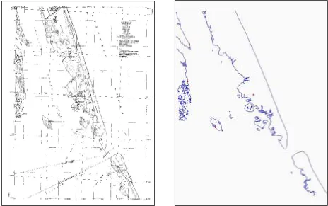
coverages. Shown in Figure 4-2 are the scanned raster and vectorized versions of T-sheet
T9278, which covers the southern end of Bodie Island.
The NOAA project has resulted in digital T-sheet shorelines for virtually all of the North
Carolina coast. Dates for these T-sheets range from 1933 to the 1970s, though there are
frequently multiple T-sheet shorelines for a given location. The entire state, with the
exception of Currituck County, is covered by a T-sheet of a date between 1933 and 1952. It
is this shoreline that is being using in North Carolina’s current erosion rate update, as
described in Section 1.3. In the current T-sheet data set, only a December 1, 1949 shoreline
exists for the study area. This T-sheet, T9278, was originally produced at a scale of
1:20,000.
The accuracy of the shoreline on sheets is dependent on the era in which the
T-sheet was produced. Those created prior to 1941 are subject to a maximum error of +/- 0.4
inches [1 mm] at map scale, which translates to +/- 66 feet [20 meters] at a scale of 1:20,000
(Shalowitz, 1964). All maps created since 1941 meet or exceed the National Map Accuracy
Standards (NMAS) of 1941. The NMAS states:
For maps on publication scales larger than 1:20,000, not more than 10 percent of the points tested shall be in error by more than 1/30 in [0.846 mm]
measured on the publication scale; for maps on publication scales of 1:20,000 or smaller, 1/50 in [0.508 mm]. These limits of accuracy shall apply in all cases to positions of well-defined points only. Well-defined points are those that are easily visible or recoverable on the ground, such as the following: monuments or markers, such as benchmarks, property boundary monuments; intersections of roads, railroads, etc.; corners of large buildings or structures (or center points of small buildings); etc.
The NMAS has set even stricter standards for T-sheets, since they are used in navigation.
Under these stricter rules, the shoreline at map scale must always be correct within 0.2 inches
[0.5 mm] and points used in navigation must be correct within 0.1 inches [0.3 mm] (Ellis,
1978). At a scale of 1:20,000, this translates into a maximum error of +/- 33 feet [10 meters]
maximum allowable errors, a number of studies have evaluated the accuracy of historical
T-sheets. Everts, Battley, and Gibson (1983) checked 36 point and shoreline features, and
found that the NMAS standards were exceeded by all. For a study site in Delaware, Galgano
(1989) found that errors in shoreline position did not exceed 10 feet [3 meters] at a scale of
1:20,000.
The error defined by NMAS was applicable to the original paper maps. Additional
error was introduced when NOAA scanned and georeferenced the paper maps. This resulted
in a different error for each T-sheet, depending on the quality and quantity of control points
available in the georeferencing procedure. The metadata for T9278 reported a horizontal
positional accuracy of 0.587 feet [0.179 meters] for x-coordinates, and 2.00 feet [0.609
meters] for y-coordinates. Thus, the composite root mean square error (RMSE) is 2.08 feet
[0.635 meters]. The maximum potential error for T9278 is additive, and therefore 34.9 feet
[10.64 meters].
4.4. Newly Acquired Photography
An effort was made to acquire unrectified historical aerial photography for the study
area. Since the resulting positions and erosion rates were to be compared with rates found
with the COAST data, it was desirable to find photos that covered a time span at least as long
as that of the COAST data set. Additionally, finding the original photography used in the
creation of the COAST data would afford a direct comparison between historical and modern
rectification techniques. With these criteria in mind, a search was made for available
photography. The final set of photography acquired for use in this study is summarized in
Table 4-2. Aerial photography acquired for rectification.
Date of Photography
Photo Scale
Photo numbers Notes
March 14, 1962 1:12,000 128,130-135 One day from COAST date December 5, 1962 1:6,000 79-85 Eight days from nearest COAST date November 6, 1972 1:12,000 136-143 No nearby COAST date
October 21, 1980 1:12,000 3874-3876,3879 Same as COAST date September 19, 1984 1:24,000 271-275 Same as COAST date October 1, 1986 1:12,000 63-69 Same as COAST date June 17, 1992 1:12,000 646-655 Same as COAST date
All photos were used as 9 inch by 9 inch black and white prints. With the exception of the
1972 photos, each of the seven sets of photography chosen for rectification was very close in
date to a shoreline in the COAST database. Other than the 1972 photos, the largest
discrepancy in date was eight days, between the COAST date of December 5, 1962 and the
5. METHODOLOGY 5.1. Image Processing
The image processing portion of the study involved scanning, rectifying, and
mosaicking the aerial photographs. Figure 5-1 is a flowchart that summarizes the major
operations within the image processing procedure. Each specific operation in the flowchart
is explained in detail in the paragraphs that follow.
Each of the 9”x9” aerial photos was first scanned at 1200 dpi using an EPSON
Expression 1640XL flatbed scanner. Previous coastal studies used a wide range of scanning
resolutions, including 400dpi (Hiland et al., 1993), 725dpi (Moore, 2000), and 1693dpi (Overton and Fisher, 1996). Such a variation implied that resolutions have been chosen
based on available disk space and time, with little consideration given to photogrammetric
standards. It has been suggested that scanned image quality does not increase substantially
beyond a magnification level of five (Greve, 1996). When this magnification level of five
was applied to the photos in this study, the resulting scanning resolution was 1200dpi. This
was within the range of resolutions used by most organizations in the photogrammetric field
(Johnston, 2002). Experience suggested that a scanning resolution much higher than 1200dpi
would result in exceedingly large file sizes and processing times. When the scanning
resolution and the photo scale are known, the resulting pixel size, in inches, was calculated
by dividing the scale denominator by the resolution. Table 5-1 lists the pixel sizes for each
of the photos used in this study. As a comparison, the 1998 orthophotography, which was
used as ground control, was produced with a half-foot pixel size. Immediately following the
scanning, each image was cropped and saved as an uncompressed TIFF file. File sizes
Table 5-1. Pixel size for scanned photos.
Photo date Photo scale Scanning resolution/Pixel size Ground pixel size
March 14, 1962 1:12,000 1200dpi/21 microns 0.83 feet December 5, 1962 1:6,000 1200dpi/21 microns 0.42 feet November 6, 1972 1:12,000 1200dpi/21 microns 0.83 feet October 21, 1980 1:12,000 1200dpi/21 microns 0.83 feet September 19, 1984 1:24,000 1200dpi/21 microns 1.67 feet October 1, 1986 1:12,000 1200dpi/21 microns 0.83 feet June 17, 1992 1:12,000 1200dpi/21 microns 0.83 feet
The general procedure for creating a rectified mosaic from individual scanned
photographs requires successively establishing three types of orientation: interior, exterior,
and absolute. Interior orientation is established once the focal length of the camera and the
location of the principal point are known (Mikhail et al., 2001). Exterior orientation is defined by knowing the positional (x,y,z) and rotational (phi, omega, kappa) coordinates for
the camera at the moment of photography (Slama, 1980). Once interior and exterior
orientations are known, absolute orientation can be established by relating the coordinates in
the image space of the photo to real-world ground coordinates. A fourth type of image
orientation, relative orientation, refers to using two images of the same ground area to
stereoscopically create a three-dimensional representation.
For each of the seven dates of photography, a block file was created in ERDAS
Imagine OrthoBASE. The block file, analogous to the project file in ArcView, stored the file
references to all image files and provides an interface in which to conduct all following steps.
The block file required that the camera type and camera focal length are specified. Since
little camera information was known, a “frame camera” was chosen as the camera model. In
fiducials. A focal length of 6 inches [152 mm] was specified for all dates of photography,
unless written information on the photos indicated otherwise. As the focal length of the
camera for the few photos that did have camera information, 6 inches was a reasonable guess
for the remaining photos. The focal length and the digitized fiducials were sufficient for
Imagine to determine the interior orientation. Pyramid layers were then created for each
image, which allow for faster image viewing at variable scales (ERDAS website, 2002).
This automated procedure required each image to successively be resampled at a larger pixel
size. For example, pyramid creation at a power of 2 would required that an image at a
resolution of 1200dpi was resampled at resolutions of 600dpi, 300dpi, 150dpi, etc.
Prior to establishing ground control for the photos, it was necessary to properly
reference the images to each other. This was done through Imagine’s Automatic Tie Point
Collection tool. Rather than the traditional method of manually identifying several points
common to overlapping photographs, the software automatically searched and aligned groups
of like pixels on different images. Establishing the interior orientation of each image was a
prerequisite to running this tool. The Automatic Tie Point Collection Tool also required two
manually selected tie points for each overlap area in the block of images. For example, the
December 5, 1962 photography required that two common points be identified on image
pairs 79 and 80, 80 and 81, 81 and 82, and 82 and 83. Thus, a total of 8 tie points for the
block had to be selected. The Automatic Tie Point Collection Tool was then run, using the
default values for the strategy parameters such as search size, correlation size, and least
square size. The maximum number of points per image was set to be 50. The number of
resulting tie points was dependent on photo quality and the amount of overlap, but was
would have been a prohibitively time-consuming process. All tie points were then inspected
for error. The few erroneous points were deleted. In a few cases, an insufficient number of
tie points were found, and additional points had to be chosen manually. Unless they were
needed, the initial two points selected on each image pair were always deleted, with the
assumption that computer generated tie points were more accurate than those chosen
manually. Table 5-2 lists the number of tie points that were used on each image. This
number reflects all manually chosen and computer generated points that were used in the
final product. It should be noted that, due to a glossy finish on the 1972 photos, Imagine was
unable to automatically generate tie points. In this case, between 5 and 8 tie points for each
photo pair were chosen manually.
Table 5-2. Number of tie points per photo pair.
Photo Date Image Pair Number of tie points
March 14, 1962 128-130 48
130-131 23 131-132 18 132-133 23 133-134 6 134-135 39 December 5, 1962 79-80 24
80-81 21 81-82 26 82-83 9 83-84 45 84-85 30 November 6, 1972 136-137 8
137-138 8 138-139 5 139-140 5
140-141 5
141-142 5
Table 5-2. Number of tie points per photo pair.
Photo Date Image Pair Number of tie points
October 21, 1980 3874-3875 53
3875-3876 9 3876-3879 39 September 19, 1984 271-272 34
272-273 17 273-274 20 274-275 37 October 1, 1986 63-64 41
64-65 10 65-66 18 66-67 19 67-68 28 68-69 44 June 17, 1992 646-647 48
647-648 18 648-649 24 649-650 23 650-651 24 651-652 23 652-653 23 653-654 26 654-655 46
Once the tie points for a block were finalized, each image has been successfully referenced to
the others in the block.
The next procedure was to georeference this tied strip of images to real world
coordinates. Traditionally, there have been several variations on this process, each with
differing levels of accuracy. Perhaps the most accurate method of identifying real world
coordinates would be collecting and specifying GPS coordinates of visible landmarks.
Modern aerial photography missions often distribute targets, shaped like Vs, on the ground
throughout the study area. GPS coordinates are collected for these targets, which are visible
can purposely be placed anywhere they are needed. This allows for a distribution of points
throughout the entire photographic area. While this method is ideal, such predetermined
coordinates for ground locations do not generally exist for historical photography. Even
recent photos frequently have become separated from the coordinates of the associated
control points. In these cases, another method for establishing ground control is required. A
basemap, with known coordinates, can be used to georeference the photography. Points on
the historical photography are matched to the same landmarks seen on the basemap. These
basemaps are frequently NOS T-sheets or USGS 1:24,000 quad sheets, due to their
nationwide coverage. The use of these basemaps is subject to the error associated with
identifying identical points on two different maps, as well as the uncertainty implicit in the
basemap. For the quad sheets, whose accuracy is governed by NMAS, the maximum
allowable error for 90% of the points is 40.0 feet [12.2 meters]. Additionally, there is almost
always a discrepancy in dates between the quad sheets and photography, which results in
further error if non-stable points, such as the estuarine shoreline or vegetation features, are
used for control. Yet another drawback is that very few common points can be identified,
due to the lack of detail on the quad sheets. For these reasons, even though USGS quad
sheets were available for the study area, 1998 orthophotography was used as a basemap to
establish ground control. These orthophotos, produced especially for North Carolina’s
erosion rate update, have a horizontal positional accuracy of 0.5 feet. This change in
basemaps represented a significant improvement over the methodology used in the creation
of the COAST database.
ERDAS Imagine provided a convenient interface for identifying ground control
and the appropriate 1998 orthophoto was displayed on the other. The user was able to zoom
into the pixel level on each photo, and click to establish common points.
Figure 5-2. Point measurement window from ERDAS Imagine.
Suitable points for ground control included road intersections, piers, and corners of structures
at ground elevation. In a few cases, when no other points were available, stable points on the
estuarine shoreline were chosen. In all cases, only points at ground level were used. The use
of rooftops, tops of telephone poles, or any other points with significant elevation would
introduce error due to relief displacement, as discussed in Section 2-2. For obvious reasons,
points were more plentiful in the recent photography than in the 1960s photography.
ERDAS recommends choosing two ground control points (GCPs) for every third image in a
each date. ERDAS also notes that the GCPs would ideally be evenly distributed across the
photograph to accurately model the camera. Since most development in this study area
occurs along a north-south highway, points chosen in each photo were usually evenly
distributed in the north-south direction, but not necessarily from east to west. This would be
cause for concern if the shoreline was consistently on the edge of the photos. However, since
this is a narrow barrier island, there is a very small horizontal distance between the highway
and the shoreline. Table A-1 lists coordinates and descriptions of all chosen ground control
points. Each GCP must have a vertical elevation associated with it. Ideally, these elevations
would be automatically extracted from a Digital Elevation Model (DEM). Since historical
elevation data did not exist for the study area, all GCP elevations were set to zero. In an area
with highly variable topography, this would be cause for concern. On a barrier island with
all elevations less than about 10 feet, this likely introduced only a negligible amount of error
(Gorman et al., 1998; Stafford and Langfelder, 1971).
Once the GCPs and tie points were established, the software ran a block triangulation
procedure and estimated the exterior orientation parameters for each image. Each image had
6 such parameters associated with it: x, y, and z (positional elements of the camera at the
moment of photography); and omega, phi, and kappa (rotational elements of the camera at
the moment of photography). Omega is the rotation around the photographic x-axis, phi is
the rotation around the photographic y-axis, and kappa is the rotation around the
photographic z-axis (ERDAS website, 2002). The identification of these exterior orientation
parameters finalized the information that Imagine needed to complete the rectification
procedure. Once a triangulation is accepted, a transformation equation is applied to each
orientation information with each image. These calibrated images were then mosaicked into
one, using the default cutlines provided by Imagine. The cell size, which must be specified
for the resampled image, was left at the recommended value in order to avoid loss of data.
At this point, the individual rectified images for a date have been combined into one nearly
seamless image, which was referenced to real-world ground coordinates. This image was
saved as an uncompressed TIFF 6.0 file, frequently over one gigabyte in size. Figure 5-3 is
an example of a finished photo mosaic (September 19, 1984) and a close-up of the
intersection of individual photographs within the mosaic. Photo mosaics with ground control
points are included as Figures A-1 through A-7 in Appendix B. Within a mosaic, differences
between the photos can be seen due to the change in wave and sun conditions, but the
shoreline and other land features are continuous.
5.2. Shoreline Identification
There are a number of possible features on the subaerial beach that can be interpreted
as a shoreline. These include the swash terminus, mean low water, high water line, and berm
line. In order to minimize the error associated with comparing shorelines of different dates,
the same interpretation must be consistently applied. Three requirements have been
identified that are essential for shoreline recognition on aerial photography (Doaln, 1978):
1) the shoreline must be easily and consistently recognizable
2) the shoreline must be linearly continuous
3) positional variations across the beach due to changes in water level must be at a
minimum
Of nine possible shoreline interpretations listed by Dr. Dolan, only the high water line
(HWL) meets all three criteria. The high water line is defined as the limit of variable wave
runup on the beach slope (Langfelder et al., 1970). However, without knowing the tide and wave conditions at the moment of photography for each study date, it was impossible to
specifically delineate the high water line on the low quality photographs. For this reason, the
wet/dry line was used as an approximation of the high water line. The wet/dry line is
reestablished at each high tide based on the beach slope and the current wind and tide
conditions (Dolan et al., 1978). Thus, it actually represents a time average of the high water line (Overton and Fisher, 1996). The wet/dry line is seen on the aerial photograph as a
Figure 5-4. Digitized wet/dry line.
This difference in gray tone is caused by differences in the water content of the sand on
either side of the line (Langfelder et al., 1970). It has been shown that the wet/dry line closely approximates the HWL (Moore, 2000). All pre-existing shorelines used in this study
(NOS T-sheets, COAST data) represented the high water line. For this reason, as data was
created in this study, the wet/dry line was digitized as the shoreline.
The wet/dry line was digitized on each finished photo mosaic in ArcView 3.2. In
accordance with the procedure used in North Carolina’s 1998 erosion rate update, the
shoreline was digitized mostly at a scale of 1:600, with zooming in and out taking place as
5.3. Erosion Rate Calculation
There are a number of data analysis techniques that can be used to compute shoreline
erosion rates. An informed decision on the technique used is essential, since the type of data
analysis can be responsible for much of the potential variability in the calculation of rates
(Crowell and Buckley, 1992). The most prevalent, an endpoint method of rate calculation
(EP), is used by more than two-thirds of agencies that use shoreline data to manage coasts
(Fenster and Dolan, 1994). This method computes a rate by simply taking the net difference
between two shoreline positions and dividing it by the time interval between the dates of the
two shorelines. The endpoint method has been shown to produce a highly variable prediction
depending on which two shorelines are used (Honeycutt et al., 2001). The North Carolina DCM is one of the agencies that uses rates found by the endpoint method for policymaking.
Despite the availability of shorelines of several intermediate dates, the erosion rates used by
the DCM have been computed solely from the earliest shoreline position in the COAST
database and the current position (Benton et al., 1997). Within this study area, for example, the official rate in the 1992 erosion rate update was calculated using shoreline positions from
July 1, 1945 and June 17, 1992. A second method for calculating rates is through linear
regression (LR). With linear regression, a line is fit to multiple shoreline positions that
minimizes the sum of the squares of the differences between measured and calculated
shoreline positions. Linear regression potentially reduces the impact of one or two
anomalous values on the accuracy of the calculated rate (Honeycutt et al., 2001). However, regression can be sensitive to uneven point distribution and point clusters (Foster and Savage,
1989). In order to ensure meaningful results, shorelines used in regression should be well