ABSTRACT
TAGHIYEH, SAJJAD. Time Series Forecasting Using Machine Learning: Development and Extensions. (Under the direction of Robert B. Handfield and Michael G. Kay.)
This dissertation addresses two time series forecasting tasks:improving time series forecasting
accuracyandtime series forecasting model selection. In both problems, machine learning techniques
are used to achieve the goal. The first problem is investigated using a hierarchical forecasting
per-spective. The goal is to improve the parent level forecasting accuracy using child level forecasts in a
multi-level hierarchical environment. To achieve this goal, a multi-phase hierarchical forecasting
model is proposed, which uses multi-feature input to build machine learning models on the child
level of the hierarchy and uses them towards improving the forecasts at the parent level of the
hierarchy. The contribution of this project is twofold: 1- Developing a multi-phase hierarchical
procedure based on machine learning techniques, which uses multi-feature input to improve the
parent level forecast based on predictions at the child level. To the best of our knowledge, this
approach is new in literature and shows significant improvement comparing to previous
meth-ods. 2- Introducing a new hyper-parameter optimization technique by combining theHyperOpt
method andsuccessive halving, which is used in the parameter tuning phase of machine learning
models. The proposed approach is tested by using the data provided by MonarchFx corporation (a
distributed logistics solutions provider), which resulted in a significant improvement comparing to
the traditional approaches.
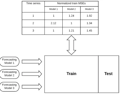
In the second problem, the focus is on selecting the best time series forecasting model among
existing ones. As opposed to traditional methods, in which a training set is used to train the
fore-casting model, and the best model is chosen based on its performance on the validation set, we
propose to use both train and validation sets holistically. In the new algorithm, train and validation
sets are used to build an intermediate classification model. This model is then used to select the
best forecasting model using the combination of train and validation sets as input to the model.
To the best of our knowledge, this work is the first in literature, which looks at time series model
selection in a different way and uses the intermediate classification for choosing the best model.
The performance of the proposed method is tested using two sources, monthly time series from
numerical experiments, seven popular time series forecasting models were used as our benchmark,
namely, naïve forecasting, moving average, exponential smoothing, ARIMA, Holt, Holt-Winters, and
Theta. Numerical results show the superiority of the new intermediate classification approach over
traditional methods.
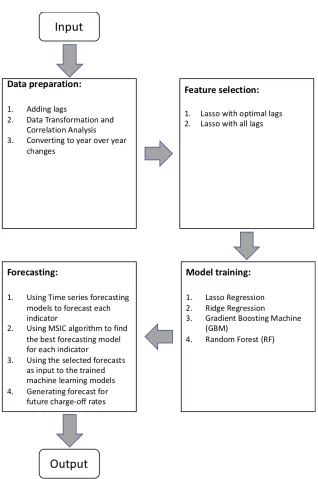
In chapter 4, we aim to use machine learning models to build a loss forecasting framework using
macroeconomic indicators. This framework consists of four components, namely, data preparation,
feature selection, machine learning training, and forecasting. We will employ Lasso regression, Ridge
regression, gradient boosting machine, and random forest as the benchmark models to develop the
loss forecasting framework. The MSIC algorithm developed in chapter 3 will be used to find the best
forecasting model for each macroeconomic indicator. The loss rate from the top 100 banks in the
US ranked by assets is used as the response variable to implement our proposed loss forecasting
framework. The macroeconomic indicators that are used as an independent variable are selected
based on a thorough review of the literature and experts’ opinions. These indicators cover consumer,
business, and government segments of the economy. The results, along with statistical summaries,
are reported, and the final numerical experiments show promising results for prediction accuracy
© Copyright 2020 by Sajjad Taghiyeh
Time Series Forecasting Using Machine Learning: Development and Extensions
by Sajjad Taghiyeh
A dissertation submitted to the Graduate Faculty of North Carolina State University
in partial fulfillment of the requirements for the Degree of
Doctor of Philosophy
Industrial Engineering
Raleigh, North Carolina
2020
APPROVED BY:
Donald Warsing Eda Kemahlioglu-Ziya
Robert B. Handfield Co-chair of Advisory Committee
Michael G. Kay
DEDICATION
BIOGRAPHY
Sajjad Taghiyeh is a Ph.D. student in the Industrial Engineering Graduate Program at North Carolina
State University. He was born in Yazd, Iran. He has received his Bachelor of Science degree in
Industrial Engineering from Sharif University of Technology in May 2013. He then came to United
States in August 2013, and he received his Master of Science degree in Operations Research from
George Mason University in December 2015. To further his education, he joined the Industrial
ACKNOWLEDGEMENTS
This dissertation would have not been completed without the guidance, help, and support I received
from my mentors, friends, and my family.
First and foremost, I am grateful for all my advisors’ guidance and their confidence in me: Dr.
Robert B. Handfield, Dr. Michael G. Kay and David C. Lengacher, who provided opportunities for me
to express my ideas and learn from my mistakes. I thank Dr. Eda Kemahlioglu-Ziya and Dr. Donald P.
Warsing who agreed to be on my committee. Their thoughtful comments on my work helped me to
improve this research.
I also would like to extend my thanks to all the faculties and staffs of the Department of Industrial
and Systems Engineering at North Carolina State University who contributed to my education.
I dedicate this work to my parents Fateme and Hossein, my wife, Foujan, and my siblings Emad
and Amir Mohammad. I appreciate their endless support and encouragement throughout my
education. This dissertation is the result of the hard days far away from home. My wish is to see
them soon.
Lastly, my friends have always been there for me, through my ups and downs, and supported me
as I traveled along this journey. Their friendship is so valuable to me and so deserve my wholehearted
thanks: Bahman Pedrood, Iman Vasheghani Farahani, Hossein Tohidi, Amirreza Sahebi fakhrabad,
TABLE OF CONTENTS
LIST OF TABLES . . . vii
LIST OF FIGURES. . . ix
Chapter 1 INTRODUCTION . . . 1
1.1 Background . . . 1
1.2 Time series forecasting . . . 2
1.2.1 Traditional time series forecasting . . . 3
1.2.2 Machine learning for time series forecasting . . . 8
Chapter 2 A Multi-Phase Approach for Product Hierarchy Forecasting in Supply Chain Management: Application to MonarchFx Inc. . . . 15
2.1 Introduction . . . 16
2.2 Literature Review . . . 17
2.3 Multi-Phase Hierarchical Forecasting Approach . . . 21
2.3.1 Overview of Forecasting Methods . . . 22
2.3.2 MPH Algorithm . . . 22
2.3.3 Hyperparameter Optimization . . . 24
2.4 Numerical Experiment . . . 27
Chapter 3 Forecasting Model Selection Using Intermediate Classification: Application to MonarchFx Corporation . . . 31
3.1 Introduction . . . 32
3.2 Literature Review . . . 35
3.2.1 Model Selection . . . 35
3.2.2 Measuring forecast error . . . 39
3.3 Model Selection Using Intermediate Classification (MSIC) . . . 41
3.3.1 Traditional forecasting model selection procedure: . . . 41
3.3.2 Proposed model selection procedure: . . . 42
3.3.3 Model Selection Using Intermediate Classification (MSIC) Algorithm: . . . 45
3.4 Numerical Experiment . . . 47
3.4.1 Extrapolative forecasting models: . . . 47
3.4.2 Results for M3-Competition Dataset . . . 48
3.4.3 Case study in MonarchFx corporation . . . 55
Chapter 4 Loss Rate Forecasting Framework Based on Macroeconomic Changes: Appli-cation to US Credit Card Industry . . . 58
4.1 Introduction . . . 59
4.2 Literature Review . . . 63
4.3 Methodology . . . 70
4.3.1 Interpretability vs accuracy . . . 70
4.3.2 Loss Forecasting Algorithm . . . 75
4.4 Numerical Experiments . . . 78
4.4.1 Data Preparation . . . 80
4.4.2 Feature Selection . . . 83
4.4.4 Forecasting . . . 88
Chapter 5 Conclusions and Future Research . . . .101
5.1 Future Research . . . 104
BIBLIOGRAPHY . . . .106
APPENDIX . . . .121
LIST OF TABLES
Table 2.1 PhaseI child-level results . . . 28
Table 2.2 PhaseI Parent level results . . . 28
Table 2.3 PhaseI I results . . . 28
Table 2.4 Top-down vs MPH MAE . . . 29
Table 2.5 Bottom-up vs MPH MAE . . . 29
Table 2.6 Comparing results of MPH to forecasts from machine learning models . . . . 29
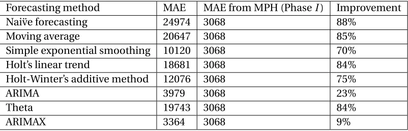
Table 2.7 Comparing phaseI results of MPH to traditional time series forecasting methods . . . 30
Table 2.8 Comparing phaseI I results of MPH to traditional time series forecasting methods . . . 30
Table 3.1 M3-Competition dataset description . . . 48
Table 3.2 Comparing the performance of MSIC to traditional train/validation model selection procedure using "Demographic" time series from M3-Competition dataset . . . 50
Table 3.3 Comparing the performance of MSIC to traditional train/validation model selection procedure using "Finance" time series from M3-Competition dataset 50 Table 3.4 Comparing the performance of MSIC to traditional train/validation model selection procedure using "Industry" time series from M3-Competition dataset 50 Table 3.5 Comparing the performance of MSIC to traditional train/validation model selection procedure using "Micro" time series from M3-Competition dataset 51 Table 3.6 Comparing the performance of MSIC to traditional train/validation model selection procedure using "Macro" time series from M3-Competition dataset 51 Table 3.7 Comparing the performance of MSIC to traditional train/validation model selection procedure using Dataset provided MonarchFx corporation . . . 56
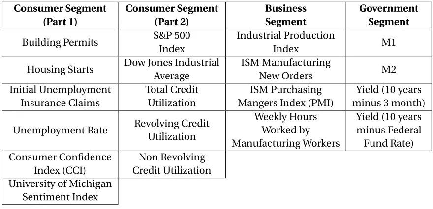
Table 4.1 List of macroeconomic indicators used in this study for building the loss forecasting framework. . . 79
Table 4.2 Results of correlation analysis and their statistical significance for economic indicators using different lags . . . 84
Table 4.3 Selected indicators using Lasso regression and optimal lags . . . 84
Table 4.4 Selected indicators using Lasso regression and all lags . . . 86
Table 4.5 Summary statistics for machine learning models when using indicators with optimal lags . . . 86
Table 4.6 Coefficients and relative importance for machine learning models when using indicators with optimal lags. . . 87
Table 4.7 Summary statistics for machine learning models when using indicators with all lags . . . 88
Table 4.8 Coefficients and relative importance for machine learning models when using indicators with all lags. . . 89
Table 4.9 Comparing the performance of MSIC to traditional train/validation model selection procedure using "Building Permits" data . . . 92
Table 4.11 Comparing the performance of MSIC to traditional train/validation model selection procedure using "M1" data . . . 92 Table 4.12 Comparing the performance of MSIC to traditional train/validation model
selection procedure using "M2" data . . . 93 Table 4.13 Comparing the performance of MSIC to traditional train/validation model
selection procedure using "Purchasing Managers Index (PMI)" data . . . 93 Table 4.14 Comparing the performance of MSIC to traditional train/validation model
selection procedure using "Weekly Hours Worked: Manufacturing" data . . . . 93 Table 4.15 Comparing the performance of MSIC to traditional train/validation model
selection procedure using "Unemployment Rate" data . . . 94 Table 4.16 MSE for predictions resulted from two feature selection approaches (optimal
lags and all lags). For each approach, MSE values are reported when using three different variants of MSIC as forecasting model selection procedure . . . 99
Table A.1 Reference list for macroeconomic indicators used in chapter 4 of this study for building the loss forecasting framework. . . 123 Table A.2 The granularity of each macroeconomic indicator along with the method we
LIST OF FIGURES
Figure 1.1 An example of time series. Performance of S&P 500 index fund in the past 90 years. Vertical bars show the recession periods in United States economy 3 Figure 1.2 A simple MLP network with 4 input nodes, 1 hidden layer with 5 hidden
nodes and 1 output . . . 13
Figure 2.1 PhaseI of MPH forecasting model . . . 24
Figure 2.2 PhaseI I of MPH forecasting model . . . 26
Figure 2.3 Proposed hyperparameter optimization algorithm. . . 26
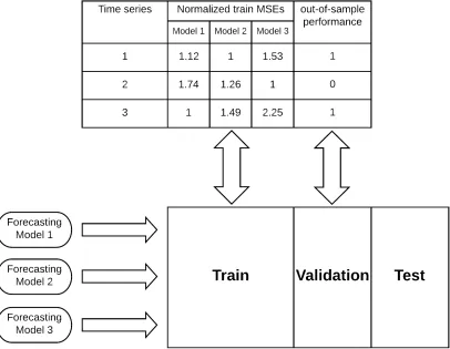
Figure 3.1 Classifier training procedure for each forecasting model in MSIC algorithm . 43 Figure 3.2 Forecasting model selection procedure in MSIC algorithm . . . 44
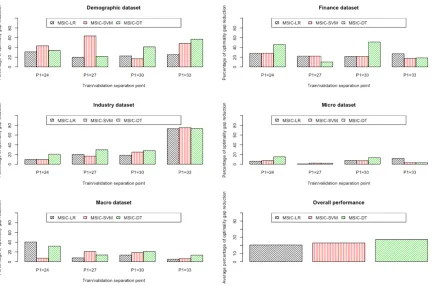
Figure 3.3 Performance comparison using "Demographic" time series from M3-Competition Dataset . . . 52
Figure 3.4 Performance comparison using "Finance" time series from M3-Competition Dataset . . . 52
Figure 3.5 Performance comparison using "Industry" time series from M3-Competition Dataset . . . 53
Figure 3.6 Performance comparison using "Micro" time series from M3-Competition Dataset . . . 53
Figure 3.7 Performance comparison using "Macro" time series from M3-Competition Dataset . . . 53
Figure 3.8 Optimality gap improvement for all categories in monthly M3-Competition data using three versions of MSIC. Average improvements for all three ver-sions over all categories are shown in last figure. . . 54
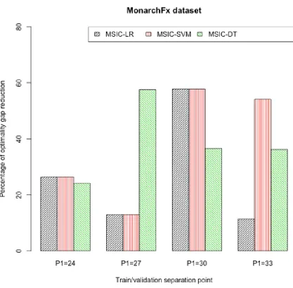
Figure 3.9 Performance comparison using dataset provided by MonarchFx corporation. 56 Figure 3.10 Optimality gap improvement for MonarchFx data using three versions of MSIC. . . 57
Figure 4.1 Steps to develop the proposed loss forecasting framework . . . 76
Figure 4.2 Consumer related macroeconomic indicators (part 1) . . . 81
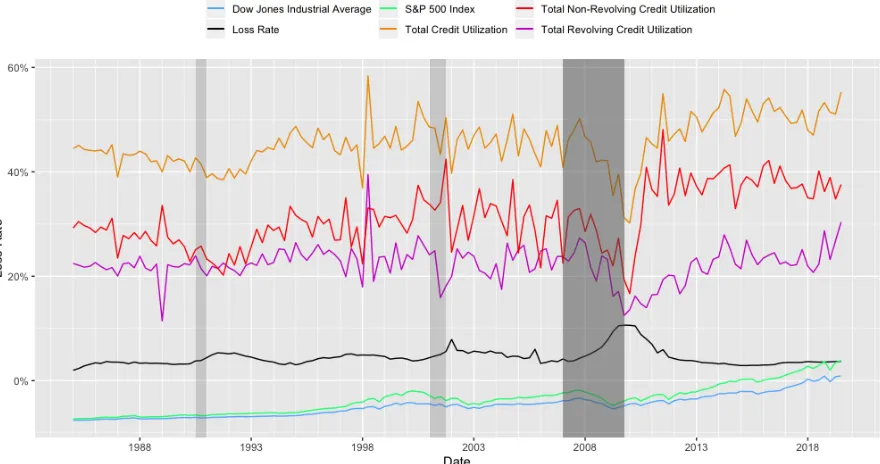
Figure 4.3 Consumer related macroeconomic indicators (part 2) . . . 81
Figure 4.4 Manufacturing related macroeconomic indicators . . . 82
Figure 4.5 Government related macroeconomic indicators . . . 82
Figure 4.6 Final fits for machine learning models using optimal lags as input variables . 87 Figure 4.7 Final fits for machine learning models using all lags as input variables . . . 89
Figure 4.8 Performance comparison using "Building Permits" Data . . . 94
Figure 4.9 Performance comparison using "Initial Unemployment Insurance Claims" Data . . . 95
Figure 4.10 Performance comparison using "M1" Data . . . 96
Figure 4.11 Performance comparison using "M2" Data . . . 96
Figure 4.12 Performance comparison using "Purchasing Managers Index (PMI)" Data . . 97
Figure 4.13 Performance comparison using "Weekly Hours Worked: Manufacturing" Data 97 Figure 4.14 Performance comparison using "Unemployment Rate" Data . . . 98
CHAPTER
1
INTRODUCTION
1.1
Background
Forecasting is a vital problem in many fields such as economics, finance, logistics, supply chain,
and healthcare due to its importance in many types of planning and decision processes. If we
want to classify the forecasting methods broadly, we can put it in the following three categories: i)
judgmental, ii) univariate, and iii) multivariate. In judgmental forecasts, the focus is on subjective
judgment, expert knowledge, or any type of inside information that will lead to a forecast for a
specific time in the future. Delphi technique[Rowe & Wright, 1999]is probably the most famous
judgemental forecasting approach. In this method, a series of questionnaires are used to perform a
survey on a group of experts, with the goal of finding a consensus of opinion. Univariate forecasting
methods are the ones using a single series of historical data as a basis of finding a pattern to predict
the future. In most instances, these series contain a function of time or some kind of linear or higher
order trends and seasonality. Multivariate forecasts are similar to univariate methods in a sense
more than one series are involved, and they are computationally more expensive. It was empirically
shown that judgmental forecasts, like other forecasting techniques, work well on some occasions
and also do not work well in others. However, the other two categories (univariate and multivariate
methods) tend to be more powerful, as they are heavily based on statistical methods and historical
facts. Generally speaking, the above approaches could also be combined in a forecasting framework
to come up with the most accurate forecast. In this dissertation, we mostly focus on univariate and
multivariate methods, but in some instances, expert opinions were used to improve the forecasting
accuracy of the statistical method.
Another way to classify forecasting problems is to put them in the following three categories:
short-term, medium-term, and long-term. Short-term forecasting problems are the ones that focus
on predicting a few time steps ahead. These time steps can be hours, days, weeks, or even years,
depending on the data granularity. Medium-term forecasting problems often predict one to two
time steps ahead, and any longer prediction horizon will fall into the long-term forecasting problem
category. Long-term forecasts are usually used in strategic planning, whereas short and
medium-term forecasts are more widely used in many activities ranging from economic planning and demand
forecasting to weather forecasts and behavioral analysis. Short-term and medium-term forecasts rely
heavily on historical data by identifying and extrapolating the patterns. Hence, statistical methods
are the basis of these forecasting models. Most of the problems in forecasting use time series as
input, which is explained in the next section.
1.2
Time series forecasting
Time series forecasting has been widely used in many applications to reduce uncertainty about the
future and avoid losses due to a lack of knowledge about the future. A time series is a time-oriented
or chronological sequence of data points (e.g.,x1,x2, ...,xn) sampled at successive points in time
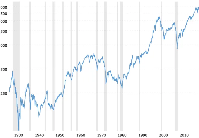
from the variable of interest. For instance, Figure 1.1 shows the values of the S&P 500 index fund in
the past 90 years, which is called a time series plot. It is common that an equally spaced time period
is selected as the rate variable.
In time series analysis, statistical methods are used to find meaningful relationships and
Figure 1.1 An example of time series. Performance of S&P 500 index fund in the past 90 years. Vertical bars show the recession periods in United States economy
forecasting focuses on developing a model to predict future based on historical patterns in already
observed time series data points. Time series forecasting can be useful in various application fields,
such as demand forecasting, finance, supply chain management, etc.[Montgomery, Johnson &
Gardiner, 1990]. There have been many models developed for time series forecasting, such as
expo-nential smoothing models[Montgomery, Johnson & Gardiner, 1990], the Box-Jenkins models[Box
et al., 2015], machine learning, and neural networks models[Dorffner, 1996]. Although a wide variety
of time series forecasting models exist, there is not a superior model that outperforms others in all
cases. Hence, investigating different models and comparing their performance is an essential task. In
the next section, an overview of time series forecasting models which were used in this dissertation
will be given. These models include both traditional and machine learning based models.
1.2.1 Traditional time series forecasting
1.2.1.1 Nai¨ve forecasting
Nai¨ve forecasting is the simplest and most cost-effective forecasting model. It is only applicable
to time series data and usually provides a basis for comparison to more complicated forecasting
x1,x2, ...,xN be the observed value at timeN and let ˆXN+hdenote the prediction for h time period
ahead (h is called forecast horizon). For nai¨ve forecasting model we have:
ˆ
XN+h=xN (1.1)
Despite the simplicity of this model, sometimes, this is the best that can be done for time series
that have complicated patterns to predict, including some financial time series. It is mostly used for
comparison to the forecasts generated by more sophisticated techniques.
1.2.1.2 Moving Average
Moving average method is one of the simplest models for time series forecasting, and it is usually
used when there exists no trend in the data. Despite its simplicity, it can be effective in many time
series forecasting tasks and is still the basis of many time series forecasting methods[Hyndman &
Athanasopoulos, 2018]. In this method, an arithmetic mean of previous observations is taken and
used as predictions for future values. LetM AN+1denote the prediction made by moving average
approach at time stepN for one step ahead. The equation for this method is as follows:
M AN+1=
PN
i=N−(n−1)xi
n (1.2)
Where n is the window of moving average and implies the number of observations used to predict.
The reason that moving average works effectively in many cases is that when an average is taken over
data, especially in time series data in which proximate observations are more likely to have similar
values, the randomness is smoothed. This way, the trend in data is captured over time, smoothed,
and applied to future forecasts.
1.2.1.3 Family of Exponential Smoothing
Exponential smoothing is a smoothing method for time series, which computes a weighted average
of past observations as the forecast. It was introduced in the 1950s[Brown, 1959; Holt, 1957;
Win-ters, 1960], and it became the basis of some of the most popular forecasting models[Hyndman &
Athanasopoulos, 2018]. Exponential smoothing provides forecasts by using the weighted averages
moving average, which gives the same weight to all the points, it assigns exponentially higher weights
to more recent observations. Forecasts generated by exponential smoothing are usually fast and
reliable, which makes them popular for industrial applications. The exponential smoothing family
consists of nine different models, among which three of them were used in this dissertation, namely
simple exponential smoothing, Holt’s linear trend method, and Holt-Winter’s additive model. We
will briefly address these three models in the following.
1.2.1.3.1 Simple Exponential Smoothing
The reason this method is called "simple" is due to the fact that it is the simplest method in
expo-nential smoothing family, and it is used in cases which no obvious trend or seasonality exists. As
discussed earlier, in Nai¨ve method, the forecast is equal to the last observed value, and in moving
average, all predictions are the average of observed values. These are two extremes in the spectrum,
and we need something in between, which is what exponential smoothing does. Despite the moving
average, in which all observed values are of equal importance, simple exponential smoothing
calcu-lates a weighted average of observations. These weights decrease exponentially as observations get
older. The recursive formula for simple exponential smoothing is as follows:
ˆ
XN+h=lN
ln=αxn+ (1−α)ln−1
(1.3)
Whereα(0≤α≤1) is the smoothing parameter, andln is the smoothed value of time series at time
n. Equation 1.3 works recursively and assigns exponentially lower weights to observations as it goes
further back in time. The above equation has two parameters (αandl0) that must be optimized.
Once these values are provided, all recursive equations can be calculated from there. However,
optimizing these values is not a trivial task, and often involves solving a non-linear minimization
1.2.1.3.2 Holt's Linear Trend Method
As discussed in the last section, in the simple exponential smoothing approach, no trend is
consid-ered for time series. To allow adding a trend variable to exponential smoothing, Holt[1957]proposed
a new recursive method, adding a new equation to smooth the trend. Following are the equations
proposed by Holt:
ˆ
XN+h=lN+h tn
ln=αxn+ (1−α)ln−1
tn=β(ln−ln−1) + (1−β)tn−1
(1.4)
Last equation is a recursive equation to add the trend to the method and smooth it over time, giving
exponentially higher weights to more recent trends in observed data.β (0≤β≤1) is smoothing
parameter for trend. Comparing to simple exponential smoothing, Holt’s linear trend method has
one more parameter ,β, to optimize.
1.2.1.3.3 Holt-Winter’s Additive Method
In Holt’s linear trend model, only trend was considered, and seasonality was ignored. To allow the
model to include seasonality, Holt[1957]and Winters[1960]introduce a new exponential smoothing
method. Let m be the frequency at which seasonality happens in a year. For example, when we
are dealing with quarterly data, m=4, and for monthly data, m=12. Following equations show the
proposed method:
ˆ
XN+h=lN+h tn+sN+h−m(k+1)
ln=α(xn−sn−m) + (1−α)(ln−1+tn−1)
tn=β(ln−ln−1) + (1−β)tn−1
sn=γ(xn−ln−1−tn−1) + (1−γ)sn−m
(1.5)
wherek=hm−1and 0≤γ≤1−α. Using Holt-Winters’ Additive method, both trend and seasonality are considered. However, it has the most parameters among all the previous methods discussed
tools.
1.2.1.4 ARIMA
ARIMA is a popular forecasting model, and it is a short form for Auto-Regressive Integrated Moving
Average. The term "autoregression" means that previous values of the same variable are used to
build the regression models, i.e., future forecast is a linear combination of previous values of the
variable of interest. An autoregressive model of orderpcould be written as:
xn=a1xn−1+a2xn−2+...+apxn−p+c (1.6)
Using past values of a variable itself makes autoregressive models able to be flexible at handling
patterns in time series. ARIMA models are the combination of differencing (computing the difference
between consecutive values) with autoregression and moving average models and are a powerful
tool in many practical forecasting problems. ARIMA model can be written as:
xn0 =a1xn0−1+a2xn0−2+...+apxn0−p+θ1εn−1+θ2εn−2+...+θqεn−q+εn+c (1.7)
Whereθi are parameters for moving average part,εi are error terms, andxi0are the differenced
series. Equation 1.7 is called an ARIMA(p,d,q) model, where p is the order of autoregressive, d is the
degree of differencing, and q is the order of moving average.
1.2.1.5 Theta
Theta model is a univariate time series forecasting model proposed by Assimakopoulos &
Nikolopou-los[2000]. Theta model proposes a decomposition of time series into short and long term
compo-nents. In this model, the local curvature of time series is modified through theta (θ) coefficient.
This coefficient is applied to the second difference of data. This way, we have a time series that
has a mean and slope similar to the original data, but the curvature is removed. Assimakopoulos &
Nikolopoulos[2000]call the modified time series "Theta-lines". In the Theta model, a time series is
decomposed into several Theta lines, which are predicted individually. After the forecasting part is
theta model at time n is as follows:
Xn e w00 (θ) =θXd a t a00
Xd a t a00 =Xn−2Xn−1+Xn−2
(1.8)
Theta model has attracted a lot of attentions after being winner of the M3-competition due to its
simplicity and predictive power, and thus is used in this dissertation as a benchmark model for
analysis.
1.2.2 Machine learning for time series forecasting
The availability of large amounts of historical data increases each day, and these data could be
used toward improving forecast accuracy. For a long time, the forecasting field was dominated
by classical models such as ARIMA. However, in the past two decades, machine learning models
have proven to be a strong competitor to classical models. Machine learning models are mostly
black-box as they rely heavily on historical data. They try to learn the stochastic relationship between
past and future by only using available data from the training set. The performance of machine
learning models has been investigated in several forecasting competitions using various datasets
[Ahmed et al., 2010; Palit & Popovic, 2006; Zhang, Patuwo & Hu, 1998]. In Werbos[1988]. It was
concluded that artificial neural networks outperform classical models in the literature, such as
linear regression and Box-Jenkins methods. Machine learning models divide into two categories,
supervised and unsupervised learning algorithms. The difference between these two categories
lies in the availability of output data. In supervised learning, we have input variables and output
variables, and the machine learning model aims to find the relationship between input and output.
However, in unsupervised learning, no output data is available, and the algorithm tries to find the
underlying hidden structure in input data in order to learn more about historical data. The problem
of forecasting time series can be tackled by supervised learning algorithms, some of which were
1.2.2.1 Multi-Linear Regression
Multi-linear regression, also known as multiple linear regression, is the most popular form of analysis
when it comes to linear regression models. As opposed to ordinary least-squares (OLS) regression,
in which only one independent variable is used to predict the response (dependent) variable, in
linear regression, more than one independent variable is used. Essentially, the goal in
multi-linear regression is to model the multi-linear relationship between the response variable and independent
variables. Multi-linear regression can be formulated as follows:
ˆ
Y =β0+β1X1+β2X2+...+βpXp (1.9)
where p is the number of predictors or independent variables, ˆY is the predicted value of response
variable,Xiis theit hindependent variable,β0is the intercept andβi,i=1, ...,p are the estimated
regression coefficients for each independent variable. Each regression coefficient (βi) estimates the
change in the response variable (Y) when changing the respective independent variable by one unit
(assuming all other independent variables have remained the same). Statistical tests are usually
performed to assess whether each regression coefficient is significantly different from 0. Following
is the assumption which multi-linear regression is based on them:
• Observations are selected randomly and independently from the population
• Residuals have a normal distribution with mean 0 and a constant variance
• Independent variables should not be highly correlated
• A linear relationship exists between the response variable and independent variables.
1.2.2.2 Ridge Regression
Ridge regression is an extension of the linear regression which uses L2 regularization to add the
L2 penalty factor to the linear model, which equals the square of the magnitude of regression
coefficients. When independent variables are highly correlated, the regression coefficient of one
variable depends on which other independent variables are included in the model. This is one
shrinks all coefficients. In Ridge regression, estimated coefficients are penalized in order to shrink
them toward zero and avoid the effects of multicollinearity. The equation for Ridge regression can
be written as follows:
Lr i d g e= n
X
i=1
(yi−xˆiβ)2+λ m
X
j=1
β2
j (1.10)
whereLR i d g eis the Ridge loss function we try to minimize andλis the regularization penalty which
requires parameter tuning. Minimizing the above equation usingβas variable, will give us estimates
for ridge regression coefficients. Note that asλ→0, βr i d g e→βO LS and asλ→ ∞, βr i d g e→0.
1.2.2.3 Lasso Regression
Least Absolute Shrinkage and Selection Operator (Lasso) is another form of regularization for linear
regression models. Similar to Ridge regression, Lasso adds a penalty term to the regular OLS model,
but instead of the L2 penalty, which is used in Ridge, Lasso adds an L1 penalty, i.e., the summation
of absolute values of regression coefficients, to OLS. The loss function for Lasso is defined as:
Ll a s s o= n
X
i=1
(yi−xˆiβ)2+λ m
X
j=1
|βj| (1.11)
As you can see from the above equation, the only difference between Ridge and Lasso lies in the
second term of their loss function. However, due to this difference, for high values ofλ, Lasso makes
many of regression coefficients equal to zero, which will result in sparse models. This is never the
case in Ridge regression.
1.2.2.4 Random Forest
Random forest is a supervised learning algorithm and is one of the most popular and easy to use
machine learning algorithms which uses an ensemble of decision trees as its building blocks to
generate the "forest". Most of the time, it can generate acceptable results even without parameter
tuning and is one of the machine learning algorithms that are less prone to overfit. Due to its
simplicity and diversity, it is one of the most widely used algorithms which can be used for both
classification and regression tasks. Random forest model combines the idea of bagging (bootstrap
each of which is trained using a subset of the training set. Each subset is generated from the original
training set using sampling with replacement (bootstrapping). After training the trees, predictions
for a new observation is made using an average over all individual regression trees. Using the bagging
technique will lead to better performance since it decreases the model’s variance without increasing
its bias. Random forest modifies the idea of bagging by adding another step to that. At each tree,
random forest selects only a random subset of features for training on the bootstrapped sample
(feature bagging). The reason to use feature bagging in the random forest is to de-correlate trees
by not allowing the selection of a dominant feature in all trees in the forest. The optimal value for
the number of trees and the depth of each tree depends on the problem and are usually treated as
tuning parameters.
1.2.2.5 Gradient Boosting Machine (GBM)
The gradient boosting machine was originally introduced to machine learning literature by Friedman
[Friedman, 2001]. Similar to the random forest, gradient boosting is an ensemble machine learning
model based upon the idea of using weak learners (usually decision trees) as building blocks for
generating a more accurate model. Unlike random forest that uses weak learners in parallel and
takes an average, GBM takes a sequential approach. It can be seen as an optimization problem to
build an additive model based on minimizing the loss function at each step. Initially, the algorithm
starts with a regular decision tree, which aims at minimizing the loss function. Then at each iteration,
it adds a new decision tree, which reduces the loss function the most. The algorithm stops when
the maximum number of iterations is reached. The mechanism of GBM is to fit decision trees to
the residuals and doing so, it improves the performance of the model in regions which it did not
perform well. GBM also haslearning rateparameter, which defines the contribution of a new tree
generated to the total model. This parameter has a range between 0 and 1, and the smaller the value
is, the more accurate the GBM model will get. However, we will incur more iterations, and the model
will be more prone to overfitting. The other way to increase the accuracy of GBM is to introduce
randomization into the fitting process[Friedman, 2002]. The randomization process which is used in
GBM is to use a randomly selected (usually without replacement) sample of the training set (instead
of using the full training set) to fit each decision tree. This is another parameter for the model that
Fernandes, 2018]:
1. Defining initial parameters: depth of decision trees (d), learning rate (α), fraction of sampling
from training set (β), and number of iterations (K)
2. Initialization: setr0=y¯ (initial residual value equals average of y[Kuhn & Johnson, 2013]) and ˆ
f =0.
3. for i=1, 2,..., K:
• select a random sample from training set according to the fractionβ(Xi,Yi).
• Use the selected sub-sample to fit a decision tree ( ˆfi) of depth d to the residuals from
previous iteration (ri−1).
• Update the model using new decision tree:
ˆ
f(x) =fˆ(x) +αfˆi(x) (1.12)
• Update residual values
ri=ri−1−αfˆi(x) (1.13)
4. Use final tree for any future predictions.
As we can see, GBM has 4 different parameters that needs tuning to achieve the best possible results.
These parameters are depth of the dection trees (d), learning rate (α),sub-sample fraction (β), and
total number of iterations (K).
1.2.2.6 Multi-Layer Perceptron (MLP)
The Multi-layer perceptron is also known as neural network and is widely used for classification and
regression tasks. Figure 1.2 shows a MLP network. Inputs are received by the network in the input
layer (first layer with four nodes in figure 1.2). In the hidden layer(s), the model tries to understand
the input data and build a relationship between input and output, and finally, in the output layer,
Figure 1.2 A simple MLP network with 4 input nodes, 1 hidden layer with 5 hidden nodes and 1 output
A simple representation of MLP model is as follows[Ahmed et al., 2010]:
ˆ y =ν0+
N H
X
j=1
νjg(ωTj x0) (1.14)
where ˆy is the network output,NHis the number of hidden layers,ν0,ν1, ...,νN H are output node
weights,x0= (1,xT)T is the input vector andωis the weight vector associated with hidden layers.
Function g is a function that determines the hidden node output. As we can see, the MLP model
has many parameters that require tuning, and there exist multiple approaches in the literature for
this task. The prominent attribute of MLP, which makes it credible, is the universal approximation
property[Leshno et al., 1993], which means that satisfying some mild conditions on functiong, any
continuous function on compact set could be approximated using an MLP with a finite number
of hidden layers. Note that the complexity of the model is determined by the number of hidden
layers, and we use k-fold cross-validation to determine this number to avoid overparametrization.
Mean squared errors are calculated to obtain the weights, and the gradient descent methods usually
optimize these weights. Back-propagation is one of the most popular algorithms for this task, which
uses the steepest decent concept.
The rest of this dissertation is organized as follows: In chapter 2,a new multi-phase hierarchical
using the information in child levels. Chapter 3 discussesa new forecasting model selection using
intermediate classification. In that chapter, a new form of forecasting model selection is proposed,
which uses the information in the training and validation sets to build a classification model to select
the best forecasting model for future predictions. Finally, chapter 4 addresses the use of machine
learning forecasting methods in the finance industry. The goal is to build a forecasting model to
predict industry loss in economic upturns and downturns based on macro-economic indicators.
The idea of chapter 3 is then incorporated in the loss forecasting model to improve the forecasting
CHAPTER
2
A MULTI-PHASE APPROACH FOR
PRODUCT HIERARCHY FORECASTING
IN SUPPLY CHAIN MANAGEMENT:
APPLICATION TO MONARCHFX INC.
Hierarchical time series demands exist in many industries and are often associated with the product,
time frame, or geographic aggregations. Traditionally, these hierarchies have been forecasted using
"top-down", "bottom-up", or "middle-out" approach. The question we aim to answer is how to
utilize child-level forecasts to improve parent-level forecasts in a hierarchical supply chain. Improved
forecasts can be used to reduce logistics costs, especially in e-commerce, considerably. We propose
a novel multi-phase hierarchical (MPH) approach. Our method involves forecasting each series in
the hierarchy independently using machine learning models, then combining all forecasts to allow
solutions provider) is used to evaluate our approach and compare it to "bottom-up" and "top-down"
methods. Our results demonstrate an 80-90% improvement in forecast accuracy using the proposed
approach. Using the proposed method, supply chain planners can derive more accurate forecasting
models to exploit the benefit of multivariate data.
2.1
Introduction
The efficient movement of goods in a supply chain depends on the ability to forecast product
de-mands accurately. Often, these forecasts must be produced within a hierarchical structure, which
may represent geographic regions, product families,[Hyndman et al., 2011], or time periods[
Athana-sopoulos et al., 2017]. The value of hierarchical forecasting is that it can provide decision support
information to different stakeholders across various organizational functions and managerial levels
[Fliedner & Mabert, 1992]. For instance, hierarchical forecasts can be used to improve market
po-sitioning, inventory planning, facility layouts, or increased efficiency of operational logistics and
transportation networks, leading to increased customer satisfaction and lower costs. Muir[1979]
explained how hierarchical forecasting can increase overall forecast accuracy, noting that combining
data from two or more homogeneous items can produce a stabilizing effect.
Two dominant approaches exist in the hierarchical forecasting literature: top-down and
bottom-up. In the top-down approach, a forecast is initially created at an aggregated level, then disaggregated
to lower levels of the hierarchy[Boylan, 2010]. A common disaggregation approach involves
prora-tion[Fliedner, 1999; Strijbosch, Heuts & Moors, 2007]in which the aggregate demand forecast is
multiplied by the ratio of corresponding demand to aggregate demand, resulting in an estimate for
the next lower level in the hierarchy. In the bottom-up approach, the steps are reversed. The lowest
level of the hierarchy is forecasted first (i.e., SKU level), then aggregated to estimate higher levels
in the hierarchy[Hyndman et al., 2011]. A third approach called middle-out combines aspects of
top-down and bottom-up. In middle-out, the forecast is performed at a middle level of the hierarchy,
then aggregated up and disaggregated down to estimate the forecasts for other levels of the hierarchy.
With respect to top-down forecasting, Gross & Sohl[1990]argued that two simple disaggregation
techniques could be effective; ”average historical proportions" and ”proportions of the historical
ap-proach, the share of each lower-level time series of the aggregated series is calculated across all
periods, i.e., a linear average share is used. In the ”proportions of the historical averages” approach,
a volume-weighted share across all time periods is employed. The authors also mention that for
the “average historical proportions” approach, one is not required only to use the historical
propor-tions, but can utilize the forecasted proportions instead. Promising results were derived using this
approach, and it is offered in some forecasting software[Boylan, 2010].
In practice, there may be multiple features in the input data (e.g., date, time, holidays, seasonal
discounts, etc.) that can be leveraged to improve forecast accuracy within supply chains. To the
best of our knowledge, most of the research in the supply chain hierarchical forecasting literature
is univariate. We found no documented multivariate hierarchical forecasting models that employ
lower-level forecasts as features in parent level modeling. In this research, we employ multiple
features (in contrast to univariate time series data) and child level (SKUs), and parent level (brand)
forecasts in a hierarchical supply chain model to improve forecast accuracy at the parent level
in the hierarchy. We utilize Machine Learning (ML) techniques including Multi-Layer Perceptron
(MLP), Random Forest (RF), Gradient Boosting (GB), and Extreme Gradient Boosting (XGB) to build
competing forecasting models. The rest of the paper is organized as follows: In section 2, we briefly
review the various existing hierarchical forecasting methods and the aggregation approaches in use.
In section 3, we present the details of our proposed Multi-Phase Hierarchical forecasting approach
(MPH). We then describe numerical experiments that demonstrate the performance of MPH using
sales data from MonarchFx Inc. (a logistics solutions provider) that is representative of a mid-tier
supply chain customer in section 4. We summarize our conclusions and discuss the practical aspects
of our work in section 5.
2.2
Literature Review
The performance of top-down and bottom-up forecasting approaches in the literature are mixed
[Syntetos et al., 2016]. Some authors found top-down approaches to be superior[Barnea &
Lakon-ishok, 1980; Fliedner, 1999; Gross & Sohl, 1990], while others found bottom-up methods to be more
accurate.[Dangerfield & Morris, 1992; Gordon, Morris & Dangerfield, 1997]. These conflicting results
products involved. To illustrate, consider a three-level product hierarchy, with product sales at the
lowest level, group sales at the middle level, and category sales at the top level. Since group sales are
determined by the sum of product sales (given the additive nature of the hierarchy), and the sum of
group sales determines category sales, the underlying demand process is transformed at different
levels of the hierarchy. When aggregating, a significant loss of information can occur, which tends
to render bottom-up forecasting more favorable. Conversely, in the top-down approach, benefits
can occur due to random noise cancellation[Fliedner, 1999]. Because the performance of each
approach depends on the demand generation process within the data, a wide range of conflicting
results appears in the literature. Thus, depending on the demand process and parameter settings,
one approach may perform better than the other in different contexts[Widiarta, Viswanathan &
Piplani, 2007, 2009].
An early study comparing both top-down and bottom-up approaches was conducted by Grunfeld
& Griliches[1960], in which they found the top-down approach more accurate, with the explanation
that disaggregated data is more susceptible to error. Fogarty & Hoffmann[1983]and Narasimhan,
McLeavey & Billington[1995]derived similar conclusions in their work. Conversely, the loss of
information in a top-down approach was considered substantial in Orcutt, Watts & Edwards[1968]
and leading to the conclusion that the bottom-up approach is superior. In Shlifer & Wolff[1979], the
authors identified conditions on the hierarchy’s structure and forecast horizon, under which they
concluded that the bottom-up approach is favorable. The robustness and bias of both approaches
were investigated in Schwarzkopf, Tersine & Morris[1988]. The authors concluded that the
bottom-up approach is more favorable unless there exist unreliable or missing data at the bottom of the
hierarchy.
A significant characteristic of the underlying demand process involves the dependencies
be-tween demand produced at each level, which can be a reason for the performance differences
between top-down and bottom-up approaches[Chen & Boylan, 2007].
Sbrana & Silvestrini[2013]summarizes the arguments that are often made against top-down
approaches. First, he states that the high (or low) variance in one level in a hierarchy may be indicative
of high (or low) variance at other levels. In such cases, allocating measures of variance from higher
levels to lower levels in a hierarchy may yield better results. Second, since different products may be
the top-down approach less appealing.
On the other hand, there are examples in the supply chain forecasting literature where the
authors favor the top-down approach. In Boylan[2010], the author found that aggregated data
can lead to more accurate sales forecasts when dealing with change policies (e.g., change in pack
sizes), compared to individual level forecasts. In such cases, common disaggregation techniques
(”average historical proportions” and ”proportions of the historical averages”) may not be useful,
and judgmental estimates are required in disaggregation methods to handle such changes in policy.
One method to overcome these drawbacks involves the analysis of the conditions in which each
approach produces superior forecasting accuracy outcomes. In Widiarta, Viswanathan & Piplani
[2008], the top-down and bottom-up approaches are compared in the context of production
plan-ning. Their goal was to estimate requirements at the SKU level. The aggregate demand series were
assumed to have correlated sub-aggregate components, each of which were assumed to follow a
first-order univariate moving average (stationary) process correlated over time. They concluded
that both methods have nearly identical performances. Later, Widiarta, Viswanathan & Piplani
[2009]investigated the relative effectiveness of bottom-up and top-down approaches to forecasting
demand at the aggregate level rather than the SKU level. They concluded that when all sub-aggregate
components of the time series follow a first-order univariate moving average process with identical
coefficients of the serial correlation term, the relative performance of both top-down and bottom-up
approaches are similar. Additionally, the different coefficients of the serial correlation term among
sub-aggregate components were examined in a simulation study. The result was that the differences
in the performance are relatively insignificant when there are small or moderate correlations
be-tween the sub-aggregate components. Sbrana & Silvestrini[2013]found that when moving average
parameters are not identical, the performance of top-down and bottom-up approaches is similar.
More recently, Rostami-Tabar et al.[2015]analyzed theoretically and by means of simulation
(using theoretically generated data) the relative performance of top-down and bottom-up
fore-casting methods for both aggregate and SKU level demand. The latter was assumed to follow a
non-stationary ARIMA (0,1,1) demand process and exponential smoothing (which is optimal for
this demand process). An important finding was that the forecast accuracy improvements achieved
by bottom-up and top-down methods for non-stationary demands are higher than those associated
from a European superstore.
A limitation observed in this work is that the generation of forecasts is dominated by the time
series at a single level of aggregation (the point at which forecasts are created). To overcome this
issue, a regression-based approach was introduced by Hyndman et al.[2011]. In their approach,
they estimated the time series at multiple hierarchy levels and then optimized this combination
using linear regression. This approach sought to derive the benefits of an ensemble of bottom-up
and top-down approaches, employing a linear combination of both. Their method demonstrated
a significant improvement in forecast accuracy compared to the traditional approaches. This
im-provement was believed to be a function of employing a combination of forecasts that reduced the
variance of forecast error[Barrow & Kourentzes, 2016; Timmermann, 2006]. Hyndman et al.[2011]
conclude that their proposed combination method is "optimal", and compared to all combination
forecasts, it leads to the least variance. Their work is inspired by earlier research in economics,
focusing on revising measurements of macro-economic indicators[Espasa, Senra & Albacete, 2002;
Hubrich, 2005; Zellner & Tobias, 2000]. Other research focuses on using different sources to combine
forecasts, e.g., utilizing different available information provided by human experts[Budescu & Chen,
2014; Lamberson & Page, 2012]. Additionally, the combination of forecasts may reduce model
speci-fication and estimation uncertainty[Kourentzes, Barrow & Crone, 2014]. In a later work, Hyndman &
Athanasopoulos[2014]demonstrate the extendibility of their combination approach for hierarchical
forecasting to non-hierarchical time series, and time series with a partial hierarchical structure.
They also proposed a solution to solve the scalability problem that existed in their previous paper
Hyndman et al.[2011]. They use a linear model structure for a more efficient coefficient estimation.
In Pennings & Dalen[2017], the authors utilize all the series in a hierarchy in contrast to a
top-down or bottom-up approach. They then incorporate a Kalman filter and state space model
to comprehend the dependencies between products (e.g., product substitution, product
comple-mentarity). Using a multivariate state space, one can estimate the hierarchical time series efficiently
using a Kalman filter as a prediction error decomposition tool[Durbin & Koopman, 2012]. In this
manner, multiple methods for forecasting hierarchical time series exist[Hyndman & Khandakar,
2008; Snyder, Ord & Beaumont, 2012]. In their approach, forecasts for the aggregate level is derived
by summing the forecast of product sales at the base level. The Kalman filter is then used to track
this manner, the forecast leverages the information from all series. The authors conclude that their
approach is superior to the traditional top-down and bottom-up approach since they incorporate
information from all levels of the hierarchy.
Our work builds on the research by Hyndman et al.[2011], and Pennings & Dalen[2017]
(dis-cussed previously), in which they combine information at all levels of hierarchy to improve
forecast-ing accuracy. However, these authors only employ univariate data as their input and do not leverage
multiple features. Our main contribution in this paper is to propose a novel approach which 1)
utilizes forecasts at lower levels to improve forecasts at higher levels, 2) uses multivariate data at
each level of the hierarchy instead of univariate data, which is more commonly seen in the literature,
and 3) leverages machine learning models. The latter component is, to the best of our knowledge,
a novel application in the supply chain forecasting literature. To achieve our goal, we propose an
MPH approach, which is discussed in the following section.
2.3
Multi-Phase Hierarchical Forecasting Approach
Our goal is to find a small loss value,l(.), in the parent level of the hierarchy, to optimize:
min
ω
1 n
n
X
i=1
l(θ(xi;ω),yi) (2.1)
Whereωis the matrix of the weights,xiis the vector of the inputs from theit hinstance,y i is
the dependent variable, e.g., demand (sales) values, andθ(.)is the output function defined by the
forecasting model. The well-known Mean Absolute Error (MAE) is being used as our loss function,
l(.), in which the average of differences between the actual demands and estimated demand is
calculated.
To achieve a higher level of accuracy in the parent level of the hierarchy, we utilize an MPH
approach. In the first phase, we forecast at both child level (SKU level), and parent level (brand)
demands using several machine learning approaches. Then, for each time series, we select the
most promising forecast method in terms of MAE. MAE is calculated based on a cross-validation
technique. In the second phase, we aggregate the forecasts at the child level and parent level and
2.3.1 Overview of Forecasting Methods
Conventional parametric forecasting techniques include ARIMA, GARCH, and TRANSFER models
[Box et al., 2015; Shumway & Stoffer, 2011]. Moreover, Taylor[2000]forecasts the demand for time
steps ahead using a normal distribution. However, in situations where demand values are volatile
and correlated over time, their model does not yield good performance. One way to overcome this
issue is to use a class of algorithms called "universal approximators". This class of algorithms is based
on machine learning techniques and is able to approximate any function given an arbitrary forecast
accuracy. These approximators can learn any function of past and future data. Therefore, other
forecasting models can be considered as a subset of the functions which they can learn. Machine
Learning (ML) techniques, such as Multi-Layer perceptron (MLP), Random Forest (RF), Gradient
Boosting (GB), and eXtreme Gradient Boosting (XGB) are some of these universal approximators,
which are able to be used to learn any function and have many applications in practice[Belgiu
& Dr˘agu¸t, 2016; Chen & Guestrin, 2016; Cigizoglu, 2004; De’Ath, 2007; Deo et al., 2018; Hippert,
Pedreira & Souza, 2001; Mei et al., 2014; Moisen et al., 2006; Rahmati, Pourghasemi & Melesse, 2016].
Supply chain forecasting is a field that generally consists of very "noisy" data. Thus it is essential
to control for noise and learn the true underlying demand patterns which are likely to be repeated
in the future. The universal approximators discussed earlier have two desirable features that make
them suitable for the supply chain forecasting problem while dealing with noise. The first is that
they are the capability of learning any arbitrary function, while the second feature is the capability
to control the learning process.
Since we want to exploit additional information provided by multiple input features, we are
faced with a multi-dimensional input data vector. The traditional parametric forecasting models
such as ARIMA are not able to integrate multi-dimensional inputs. Thus we exploit the ability of
universal approximators to take multi-dimensional inputs and utilize them in our forecasting model.
The details of the MPH approach are explained in the following subsection.
2.3.2 MPH Algorithm PhaseI:
perceptron, random forest, gradient boosting, extreme gradient boosting, etc. Suppose we
have chosenN forecasting approaches. Seti=1.
• Step 1: Use theit hforecasting approach to forecast parent level demand (brand demand) and
child level demands (SKU demand).
• Step 2: Optimize the hyperparameters of theit hforecasting method using a search approach,
e.g., Bayesian optimization method, grid search, successive halving.
• Step 3: Seti=i+1. Ifi=N+1, go to step 4. Otherwise, go to step 1.
• Step 4: Using the outputs of the previous steps, record the best forecasting approach and the
associated outputs for demands at all levels.
PhaseI I:
• Step 5: Append the recorded outputs of step 4 to input data of the parent level, as additional
features.
• Step 6: Repeat steps 1 and 2 once more, using the new input data with additional features. The
only modification is to forecast the parent level.
• Step 7: Choose the best forecasting output among the forecasting methods used in step 6.
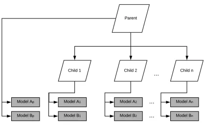
Figure 2.1 provides an overview of phaseI for this procedure, in which two forecasting models
were chosen as base forecasting approaches. Model A can be a tree-based forecasting model, e.g., RF,
GB, or XGB, and model B can represent an exploration-capable model, e.g., artificial neural network
models such as MLP. As depicted in figure 2.1, we have a two-level hierarchical structure with one
parent and n children. In phaseI of the model, we use the selected models (i.e., models A and B) to
forecast demands at both parent and child levels. Since we are dealing with universal approximators,
they have several hyperparameters, on which the model is very sensitive in term of accuracy. Hence,
one needs to find an approach to optimize the hyperparameters of the forecasting models, which is
Figure 2.1 PhaseIof MPH forecasting model
2.3.3 Hyperparameter Optimization
Several approaches in the literature address hyperparameter optimization in machine learning
[Bergstra, Yamins & Cox, 2013; Feurer, Springenberg & Hutter, 2015; Li et al., 2017; Maclaurin,
Duvenaud & Adams, 2015]. In this paper, we use the hyperOpt algorithm proposed by Bergstra,
Yamins & Cox[2013], and combine it with the successive halving approach[Jamieson & Talwalkar,
2016]to obtain a more efficient search. In the following, a summary of the HyperOpt algorithm is
provided, and the details of the proposed hyperparameter optimization algorithm are explained.
2.3.3.1 HyperOpt:
HyperOpt is a module proposed by Bergstra, Yamins & Cox[2013], and is focused on intelligently
searching through the hyperparameter space. One approach is to use the Tree-structured Parzen
Estimator (TPE) algorithm[Bergstra et al., 2011], in which the search space is explored intelligently,
while the parameter values are narrowed down to the best estimated parameters. In contrast to the
HyperOpt is an oriented random search and is proven to work efficiently[Bergstra, Yamins & Cox,
2013]. Hence, it serves as a good candidate to tune and optimize hyperparameters for universal
approximators, as adopted in this paper.
2.3.3.2 Proposed Hyperparameter Optimization Algorithm:
• Initializing the sample space by HyperOpt. Suppose that we choose to start withN parameter
settings to search more rigorously among them. In our modified approach, we use HyperOpt
to search intelligently through the search space, and we store the firstN parameter settings
that are used by HyperOpt. Note that each HyperOpt iteration is only performed on one set
of train/test data. Now we use the generatedN parameter settings as an input for a more
rigorous search by successive halving[Jamieson & Talwalkar, 2016].
• We follow the idea of successive halving proposed by Jamieson & Talwalkar[2016]. UsingN
parameter settings generated by HyperOpt, the well-known K-fold algorithm[Kohavi, 1995]
is used to evaluate each parameter settings for a fixed amount of time/budget, e.g., T. Then,
we select the top-performing half of the parameter settings(N/2), and again, we evaluate
them via k-fold for time 2T. This procedure is repeated until the search space is singular or the
designated budget is exhausted.
The idea behind the above algorithm is quite intuitive. Initially, HyperOpt is used as the
screen-ing procedure in the search region by expendscreen-ing a small budget of processscreen-ing time. After initial
candidates (parameter settings) were selected, successive halving is utilized for a more rigorous
evaluation. This procedure spends computational budget more efficiently by focusing on the parts
of the search region, which have more potential. This procedure is shown in figure 2.3.
In the second phase we add the best performing forecasts as additional features to the input
data of the parent (See Figure 2.2). Next, a parent level forecasting model is re-estimated using the
new input, and then the hyperparameter optimization process is conducted. After identifying the
Figure 2.2 PhaseI Iof MPH forecasting model
2.4
Numerical Experiment
The MPH forecasting algorithm was implemented on sales data provided by MonarchFx Inc., which
consists of 935 days of data for ten Stock Keeping Units (SKUs) and aggregated data, which represents
total brand sales. This data is representative of one of MonarchFx’s mid-tier supply chain customers.
In addition to the historical sales data, the input also contained additional features, including:
• Promotion: a binary variable indicating if a promotion was present.
• Holiday: a binary variable indicating holiday periods.
• Day of the week: seven dummy variables corresponding to day of the week.
• Date: in the format day/month/year
Each of these factors may increase the predictive power of forecasting models, both
indepen-dently as well as in combinations.
To measure model accuracy, the Mean Absolute Error (MAE) is used:
M AE =
Pn
i=1|yi−yiˆ|
n (2.2)
Whereyicorresponds to the actual values of sales, andyiˆis the forecasted sales on dayi.
The well-known k-fold cross-validation method[Kohavi, 1995]with k=5 is used to test each
forecasting model and measure the forecast accuracy. The parameter k refers to the number of
groups that we divide the input data. We chose this method because it provides a less biased estimate
of the model compared to a single train/test split of the data. In this procedure, initially, the data is
divided into k groups. Then, for each group, it is selected as the test dataset, and the remaining data
is considered as the training set. The forecasting model is trained on the train set, and the accuracy
is measured on the test set. This procedure is repeated for every group, and the average MAE across
k train/test splits is reported as the final MAE.
Multi-Layer Perceptron (MLP), Random Forest (RF), Gradient Boosting (GB), and Extreme
Gradi-ent Boosting (XGB) are the forecasting models selected for the experimGradi-ents, due to their popularity
Table 2.1PhaseIchild-level results
Series MLP RF GB XGB Best Range Min MAE
1 370 339 366 350 RF 31 339
2 404 381 405 388 RF 24 381
3 607 557 609 588 RF 52 557
4 681 684 725 708 MLP 44 681
5 364 343 389 360 RF 46 343
6 408 385 397 405 RF 23 385
7 676 691 732 709 MLP 56 676
8 446 421 449 451 RF 30 421
9 537 537 550 537 MLP 13 537
10 395 363 385 375 RF 32 363
Table 2.2PhaseIParent level results
MLP RF GB XGB Best Range Min MAE
3972 3182 3068 3118 GB 904 3068
2014; Zieba, Tomczak & Tomczak, 2016]. Using these four forecasting models, the MPH algorithm,
in conjunction with the hyperparameter optimization method (explained in section 3-2), is
imple-mented on the data, and the forecasting error at the parent level is compared to the top-down and
bottom-up approach.
Tables 2.1 and 2.2 show the results of phaseI of the algorithm for the lower level and parent
level of the hierarchy, respectively. Table 2.1 contains 10 rows corresponding to each SKU. MAE is
reported for each of four forecasting methods (after performing k-fold cross-validation), and the
forecasting method with the minimum MAE is selected for phaseI I.
The results of phaseI are added as additional features to input data at the parent level. As phase
I I of the algorithm suggests, MLP, RF, GB, and XGB models are estimated again using the new input
data. Table 2.3 reports the MAE (after performing k-fold cross-validation) at the end of phaseI I for
each of the forecasting models. The minimum MAE is selected as the final MAE at the parent level,
which is 303.
The final MAE of MPH algorithm is compared to the MAE of top-down and bottom-up approach,
Table 2.3PhaseI Iresults
MLP RF GB XGB Best Range Min MAE