Joint Tracking of Manoeuvring Targets and Classification of Their Manoeuvrability

Joint Tracking of Manoeuvring Targets

and Classification of Their Manoeuvrability

Simon Maskell

QinetiQ Ltd, St. Andrews Road, Malvern, Worcestershire WR14 3PS, UK Email:[email protected]

Department of Engineering, University of Cambridge, Cambridge CB2 1PZ, UK

Received 30 May 2003; Revised 23 January 2004

Semi-Markov models are a generalisation of Markov models that explicitly model the state-dependent sojourn time distribution, the time for which the system remains in a given state. Markov models result in an exponentially distributed sojourn time, while semi-Markov models make it possible to define the distribution explicitly. Such models can be used to describe the behaviour of manoeuvring targets, and particle filtering can then facilitate tracking. An architecture is proposed that enables particle filters to be both robust and efficient when conducting joint tracking and classification. It is demonstrated that this approach can be used to classify targets on the basis of their manoeuvrability.

Keywords and phrases:tracking, classification, manoeuvring targets, particle filtering.

1. INTRODUCTION

When tracking a manoeuvring target, one needs models that can cater for each of the different regimes that can govern the target’s evolution. The transitions between these regimes are often (either explicitly or implicitly) taken to evolve accord-ing to a Markov model. At each time epoch there is a proba-bility of being in one discrete state given that the system was in another discrete state. Such Markov switching models re-sult in an exponentially distributed sojourn time, the time for which the system remains in a given discrete state. Semi-Markov models (also known as renewal processes [1]) are a generalisation of Markov models that explicitly model the (discrete-state-dependent) distribution over sojourn time. At each time epoch there is a probability of being in one discrete state given that the system was in another discrete state and how long it has been in that discrete state. Such models of-fer the potential to better describe the behaviour of manoeu-vring targets.

However, it is believed that the full potential of semi-Markov models has not yet been realised. In [2], sojourns were restricted to end at discrete epochs and filtered mode probabilities were used to deduce the parameters of the time-varying Markov process, equivalent to the semi-Markov pro-cess. In [3], the sojourns were taken to be gamma-distributed with integer-shape parameters such that the gamma vari-ate could be expressed as a sum of exponential varivari-ates; the semi-Markov model could then be expressed as a (po-tentially highly dimensional) Markov model. This paper

proposes an approach that does not rely on the sojourn time distribution being of a given form, and so is capa-ble of capitalising on all availacapa-ble model fidelity regarding this distribution. The author asserts that the restrictions of the aforementioned approaches currently limit the use of semi-Markov models in tracking systems and that the im-proved modelling (and so estimation) accuracy that semi-Markov models make possible has not been realised up to now.

There have been some previous approaches to solving the problem of joint tracking and identification that have been based on both grid-based approximations [5] and particle fil-ters [6,7]. An important failing of these implementations is that target classes with temporarily low likelihoods can end up being permanently lost. As a consequence of this same feature of the algorithms, these implementations cannot re-cover from any miscalculations and are not robust. This ro-bustness issue has been addressed by stratifying the classi-fier [4]; one uses separate filters to track the target for each class (i.e., one might use a particle filter for one class and a Kalman filter for another) and then combines the outputs to estimate the class membership probabilities and so classifica-tion of the target. This architecture does enable different state spaces and filters to be used for each class, but has the defi-ciency that this choice could introduce biases and so system-atic errors. So, the approach taken here is to adopt a single state space common to all the classes and a single (particle) filter, but to then attempt to make the filter as efficient as pos-sible while maintaining robustness. This ability to make the filter efficient by exploiting the structure of the problem in the structure of the solution is the motivation for the use of a particle filter specifically.

This paper demonstrates this methodology by consider-ing the challengconsider-ing problem of classifyconsider-ing targets which differ only in terms of their similar sojourn time distributions; the set of dynamic models used to model the different regimes are taken to be the same for all the classes. Were one using a Markov model, all the classes would have the same mean sojourn time and so the same best-fitting Markov model. Hence, it is only possible to classify the targets because semi-Markov models are being used.

Since the semi-Markov models are nonlinear and non-Gaussian, the particle-filtering methodology [8] is adopted for solving this joint tracking and classification problem. The particle-filter represents uncertainty using a set of samples. Here, each of the samples represent different hypotheses for the sojourns times and state transitions. Since there is uncer-tainty over both how many transitions occurred and when they occurred, the particles represent the diversity over the number of transitions and their timing. Hence, the parti-cles differ in dimensionality. This is different from the usual case for which the dimensionality of all the particles is the same. Indeed, this application of the particle filter is a spe-cial case of the generic framework developed concurrently by other researchers [9]. The approach described here exploits the specifics of the semi-Markov model, but the reader inter-ested in the more generic aspects of the problem is referred to [9].

Since, if the sojourn times are known, the system is linear and Gaussian, the Kalman filter is used to deduce the param-eters of the uncertainty over target state given the hypothe-sised history of sojourns. So, the particle filter is only used for the difficult part of the problem—that of deducing the tim-ings of the sojourn ends—and the filter operates much like a multiple hypothesis tracker, with hypotheses in the (contin-uous) space of transition times. To make this more explicit, it should be emphasised that the complexity of the particle

filter is not being increased by using semi-Markov models, but rather particle filters are being applied to the problem associated with semi-Markov models. The resulting compu-tational cost is roughly equivalent to one Kalman filter per particle and in the example considered inSection 6just 25 particles were used for each of the three classes.1 _The

au-thor believes that this computational cost is not excessive and that, in applications for which it is beneficial to capi-talise on the use of semi-Markov models—which the author believes to be numerous—the approach is practically useful. However, this issue of the trade-offbetween the computa-tional cost and the resulting performance for specific appli-cations is not the focus of this paper; here the focus is on proposing the generic methodology. For this reason, a sim-ple yet challenging, rather than necessarily practically useful, example is used to demonstrate that the methodology has merit.

A crucial element of the particle filter is the proposal dis-tribution, the method by which each new sample is proposed from the old samples. Expedient choice of proposal distri-bution can make it possible to drastically reduce the num-ber of particles necessary to achieve a certain level of per-formance. Often, the trade-offbetween complexity and per-formance is such that this reduction in the number of parti-cles outweighs any additional computation necessary to use the more expedient proposal distributions. So, the choice of proposal distribution can be motivated as a method for re-ducing computational expense. Here, however, if as few er-rors as possible, are to be introduced as is critically impor-tant when conducting joint tracking and classification, it is crucial that the proposal distribution is well matched to the true system. Hence, the set of samples is divided into a num-ber of strata, each of which had a proposal that was well matched to one of the classes. Whatever the proposal dis-tribution, it is possible to calculate the probability of ev-ery class. So, to minimise the errors introduced, for each particle (and so hypothesis for the history of state transi-tions and sojourn times), the probability of all the classes is calculated. So each particle uses a proposal matched to one class, but calculates the probability of the target being a member of every class. Note that this calculation is not computationally expensive, but provides information that can be used to significantly improve the efficiency of the fil-ter.

So, the particles are used to estimate the manoeuvres and a Kalman filter is used to track the target. The particles are split into strata each of which is well suited to tracking one of the classes and the strata of particles used to classify the target on the basis of the target’s manoeuvrability. The motivation for this architecture is the need to simultaneously achieve ro-bustness and efficiency.

This paper is structured as follows: Section 2 begins by introducing the notation and the semi-Markov model

tk tk+ 1 tk+1=tk+2 tk+1+ 1

Figure1: Diagram showing the relationship between continuous time, the time when measurements were received, and the time of sojourn ends. The circles represent the receipt of measurements or the start of a sojourn.

structure that is used.Section 3describes how a particle fil-ter can be applied to the hard parts of the problem, the esti-mation of the semi-Markov process’ states. Some theoretical concerns relating to robust joint tracking and identification are discussed in Section 4. Then, inSection 5, efficient and robust particle-filter architectures are proposed as solutions for the joint tracking and classification problem. Finally, an exemplar problem is considered inSection 6and some con-clusions are drawn inSection 7.

2. MODEL

When using semi-Markov models, there is a need to distin-guish between continuous time, the indexing of the measure-ments, and the indexing of the sojourns. Here, continuous time is taken to beτ, measurements are indexed byk, and manoeuvre regimes (orsojourns) are indexed byt. The con-tinuous time when thekth measurement was received isτk. The time of the onset of the sojourn isτt;tk is then the in-dex of the sojourn during which the kth measurement was received. Similarly,kt is the most recent measurement prior to the onset of thetth sojourn. This is summarised inTable 1 whileFigure 1illustrates the relationship between such quan-tities as (tk+ 1) andtk+1.

The model corresponding to sojourntisst.stis a discrete semi-Markov process with transition probabilities p(st|st−1)

that are known; note that since, at the sojourn end, a transi-tion must occur, sop(st|st−1)=0 ifst=st−1;

regime and similarly, y1:kwill be used to denote the history of measurements up to thekth measurement.

For simplicity, the transition probabilities are here con-sidered invariant with respect to time once it has been de-termined that a sojourn is to end; that is, p(st|st−1) is not a

function ofτ. The sojourn time distribution that determines the length of time for which the process remains in statestis distributed asg(τ−τt|st):

The st process governs a continuous time process, xτ, which givenst and a state at a time after the start of the so-journxτt+1 > xτ > xτt has a distribution f(xτ|xτ,st). So, the

Table1: Definition of notation.

Notation Definition

τk Continuous time relating tokth measurement

τt Continuous time relating totth sojourn time

tk Sojourn prior tokth measurement; so thatτtk≤τk≤τtk+1 kt Measurement prior totth sojourn; so thatτkt≤τt≤τkt+1

st Manoeuvre regime forτt< τ < τt+1

distribution ofxτgiven the initial state at the start of the so-journ and the fact that the soso-journ continues to timeτis

pxτ|xτt,st,τt+1> τ

fxτ|xτt,st

. (3)

Ifxkis the history of states (in continuous time), then a probabilistic model exists for how each measurement, yk, is related to the state at the corresponding continuous time:

pyk|xk

This formulation makes it straightforward to then form a dynamic model fors1:tkprocess andτ1:tkas follows:

wherep(s1) is the initial prior on the state of the sojourn time

(which we later assume to be uniform) andp(τ1) is the prior

on the time of the first sojourn end (which we later assume to be a delta function). This can then be made conditional on

s1:tk−1andτ1:tk−1, which makes it possible to sample the semi-Markov process’ evolution between measurements:

whereA\Bis the setAwithout the elements of the setB. Note that in this case{s1:tk,τ1:tk} \ {s1:tk−1,τ1:tk−1}could be the empty set in which case,p({s1:tk,τ1:tk} \ {s1:tk−1,τ1:tk−1}|s1:tk−1,

τ1:tk−1)=1.

So, it is possible to write the joint distribution of thest andxτ processes and the times of the sojourns,τ1:tk, up to

Evolution of semi-Markov model

×pyk|xτk

Effect onxτof incomplete regimes

×

This is a recursive formulation of the problem. The an-notations indicate the individual terms’ relevance.

3. APPLICATION OF PARTICLE FILTERING

Here, an outline of the form of particle filtering used is given so as to provide some context for the subsequent discussion and introduce notation. The reader who is unfamiliar with the subject is referred to the various tutorials (e.g., [8]) and books (e.g., [10]) available on the subject.

A particle filter is used to deduce the sequence of sojourn times,τ1:tk, and the sequence of transitions,s1:tk, as a set of measurements are received. This is achieved by samplingN

times from a proposal distribution of a form that extends the existing set of sojourn times and thestprocess with samples of the sojourns that took place between the previous and the current measurements:

A weight is then assigned according to the principle of im-portance sampling:

Theseunnormalisedweights are then normalised:

wik=

and estimates of expectations calculated using the (nor-malised) weighted set of samples. When the weights become skewed, some of the samples dominate these expectations, so the particles are resampled; particles with low weights are probabilistically discarded and particles with high weights are probabilistically replicated in such a way that the expected number of offspring resulting from a given particle is propor-tional to the particle’s weight. This resampling can introduce unnecessary errors. So, it should be used as infrequently as possible. To this end, a threshold can be put on the approxi-mate effective sample size, so that when this effective sample size falls below a predefined threshold, the resampling step is performed. This approximate effective sample can be calcu-lated as follows:

It is also possible to calculate the incremental likelihood:

pyk|y1:k−1

which can be used to calculate the likelihood of the entire data sequence, which will be useful in later sections:

py1:k

4. THEORETICAL CONCERNS RELATING TO JOINT TRACKING AND CLASSIFICATION

Conversely, if the system does not forget, then errors will accumulate and this will eventually cause the filter to di-verge. This applies to sequential algorithms in general, in-cluding Kalman filters,2_{which accumulate finite precision}

er-rors, though such errors are often sufficiently small that such problems rarely arise and have even less rarely been noticed.

For a system to forget, its model needs to involve the states changing with time; it must beergodic. There is then a finite probability of the system being in any state given that it was in any other state at some point in the past; so, it is not possible for the system to get stuck in a state. Models for clas-sification do not have this ergodic property since the class is constant for all time; such models have infinite memory. Ap-proaches to classification (and other long memory problems) have been proposed in the past based on both implicit and explicit modifications of the model that reduce the memory of the system by introducing some dynamics. Here, the em-phasis is on using the models in their true form.

However, if the model’s state is discrete, as is the case with classification, there is a potential solution described in this context in [4]. The idea is to ensure that all probabilities are calculated based on the classes remaining constant and to run a filter for each class; these filters cannot be reduced in num-ber when the probability passes a threshold if the system is to be robust. In such a case, the overall filter is condition-ally ergodic. The approach is similar to that advocated for classification alone whereby different classifiers are used for different classes [13].

The preceding argument relates to the way that the fil-ter forgets errors. This enables the filfil-ter to always be able to visit every part of the state space; and the approach advo-cated makes it possible to recover from a misclassification. However, this does not guarantee that the filter can calculate classification probabilities with any accuracy. The problem is the variation resulting from different realisations of the er-rors caused in the inference process. In a particle-filter con-text, this variation is the Monte Carlo variation and is the result of having sampled one of many possible different sets of particles at a given time. Put more simply; performing the sampling step twice would not give the same set of samples.

Equation (13) means that, if each iteration of the tracker introduces errors, the classification errors necessarily accu-mulate. There is nothing that can be done about this. All that can be done is to attempt to minimise the errors that are in-troduced such that the inevitable accumulation of errors will not impact performance on a time scale that is of interest.

So, to be able to classify targets based on their dynamic behaviour, all estimates of probabilities must be based on the classes remaining constant for all time and the errors intro-duced into the filter must be minimised. As a result, clas-sification performance is a good test of algorithmic perfor-mance.

2_{It is well documented that extended Kalman filters can accumulate} lin-earisation errors which can cause filter divergence, but here the discussion relates to Kalman filtering with linear Gaussian distributions such that the Kalman filter is an analytic solution to the problem of describing the pdf.

5. EFFICIENT AND ROBUST CLASSIFICATION

The previous section asserts that to be robust, it is essential to estimate probabilities based on all the classes always re-maining constant. However, to be efficient, the filter should react to the classification estimates and focus its effort on the most probable classes (this could equally be the class with the highest expected cost according to some nonuniform cost function but this is not considered here).

To resolve these two seemingly contradictory require-ments of robustness twinned with efficiency, the structure of the particle filter can be capitalised upon. The particle fil-ter distinguishes between the proposal used to sample the particles’ paths and the weights used to reflect the disparity between the proposal and the true posterior. So, it is possi-ble for the proposal to react to the classification probabili-ties and favour proposals well suited to the more probable classes while calculating the weights for the different classes; this is equivalent to Rao-Blackwellising the discrete distribu-tion over class for each particle.

One could enable the system to react to the classification probabilities while remaining robust to misclassification by each particle sampling the importance function from a set of importance samplers according to the classification prob-abilities. Each importance sampler would be well suited to the corresponding class and each particle would calculate the weights with respect to all the classes given its sampled values of the state.

However, here a different architecture is advocated; the particles are divided into strata, such that the different strata each use an importance function well suited to one of the classes. For any particle in the jth stratum, Sj, and in the context of the application of particle filtering to semi-Markov models, the importance function is then of the form

q({s1:tk,τ1:tk}\{s1:tk−1,τ1:tk−1}|{s1:tk−1,τ1:tk−1},yk,Sj). The strata then each have an associated weight and these weights sum to unity across the strata. If each particle calculates the proba-bility of all the classes given its set of hypotheses, then the architecture will be robust. It is then possible to make the ar-chitecture efficient by adding a decision logic that reacts to the weights on the strata; one might add and remove strata on the basis of the classification probabilities. The focus here is not on designing such a decision logic, but to propose an architecture that permits the use of such logic.

To use this architecture, it is necessary to manipulate strata of particles and so to be able to calculate the total weight on a class or equally on a stratum. To this end, the relations that enable this to happen are now outlined.

The classes are indexed byc, particles byi, and the strata by j. The model used to calculate the weights isM and the stratum isS. So, the unnormalised weight for theith particle in stratumSj, using modelMc, is ¯w(

i,j,c)

k .

The weight on a stratum,p(Sj|y1:k), can be deduced from

pSj|y1:k

∝py1:k|Sj

pSj

, (14)

This leads to the following recursion: fication of (12) as follows:

pyk|y1:k−1,Sj

Similarly, for the classes,

pMc|y1:k

To implement this recursion, the weights of the classes are normalised such that they sum to unity over the particle in the strata:

These weights are then normalised such that they sum to unity within each strata:

w(ki|j)

where ¯w(kj)is the total unnormalised weight of the stratum:

¯

w_k(j)

i ¯

w_k(i,j). (22)

These weights are also normalised such that they sum to unity across the strata:

w(_kj) w¯

The skewness of each stratum is then used to assess whether that stratum has degenerated and so if resampling is necessary for the set of particles in that stratum. This means that the weight relating toMcfor theith particle within the

jth stratum is

w(ki,j,c)∝w

So, withNPparticles andNMclasses (and soNMstrata), running the algorithm overNK steps can be summarised as follows inAlgorithm 1.p(x0) is the initial prior on the state

and Implement Recursion is conducted as in Algorithm 2 whereVjis the reciprocal of the sum of the squared weights, on the basis of which one can decide whether or not it is nec-essary to Resample.NTis then the threshold on the approxi-mate effective sample size which determines when to resam-ple;NT ≈ (1/2)NP might be typical. Note that the resam-pling operation will result in replicants of a subset of some of the particles within thejth stratum, but that for each copy of theith particle in the jth stratum,w(kc|i,j)is left unmodi-fied.

6. EXAMPLE

6.1. Model

The classification of targets which differ solely in terms of the semi-Markov model governing thest process is considered. The classes have different gamma distributions for their so-journ times but all have the same mean value for the soso-journ time, and so the same best-fitting Markov model. As stated in the introduction, this example is intended to provide a diffi -cult to analyse, yet simple to understand, exemplar problem. The author does intend the reader to infer that the specific choice of models and parameters are well suited to any spe-cific application.

Thexτprocess is taken to be a constant velocity model; an integrated diffusion process

fxτ+∆|xτ,s mean,m, and covariance,C, and where

Initialise ¯wk=0 Forj=1 :NM

InitialiseVj=0

Initialise output classification probabilities: ¯Pc k=0

Resamplejth stratum if 1/Vj< NT End For

Algorithm2

where the discrete state,st, takes one of two values which dif-fer in terms ofσ2

s;σ12=0.001 andσ22=100.

The data are linear Gaussian measurements of position

pyk|xτk

andR=0.1. The measurements are received at regular inter-vals such thatτk−τk−1=0.5 for allk >1.

The three classes’ sojourn distributions are

gτ−τt|st,Mc

Figure 2: Sojourn time distributions forst = 1 for the different classes.

whereG(x;α,β) is a gamma distribution overx, with shape parameterαand scale parameterβ.Figure 2shows these dif-ferent sojourn time distributions. Note that since the mean of the gamma distribution is αβ, all the sojourn distri-butions for st = 1 have the same mean. Hence, the ex-ponential distribution (which only has a single parameter that defines the mean) for all three classes would be the same.

Since there are only two discrete states, the state transi-tion probabilities are simple:

pst|st−1

This means that, given the initial discrete state, the so-journ ends define the discrete-state sequence.

p(s1) is taken to be uniform across the two models and p(τ1) = δ(τ1−0), so it assumed known that there was a

transition at time 0.x0is initialised at zero as follows:

x0=

6.2. Tracking of manoeuvring targets

For the proposal in the particle filter, (6), the dynamic prior for thestprocess is used, with a minor modification:

qs1:tk,τ1:tk \ tended to beyondτk, but the sample of the final sojourn time is integrated out (so forgotten); the proposal simply samples that the next sojourn is after the time of the measurement, not what time it actually took place. This exploits some struc-ture in the problem sinceτtk+1has no impact on the estima-tion up to timeτk and so classification on the basis of y1:k. The weight update equation simplifies since the dynamics are used as the proposal:

¯

i_{) can straightforwardly be calculated}

by a Kalman filter with a time-varying process model (with model transitions at the sojourn ends) and measurement up-dates at the times of the measurements.

Having processed the k measurement, the ith particle then needs to store the time of the hypothesised last sojourn,

τt(ki), the current state,s

(i)

tk, a mean and covariance forxτk, and a weight,wk(i).

JustNP=25 particles are used and initialised with sam-ples fromp(s1) andp(τ1) (so all the sameτ1). Each particles’

initial value for the Kalman filter’s mean is the true initial state,m. The initial value for the covariance is then defined asC:

The weights are all initialised as equal for all the particles. Resampling takes place if the approximate effective sample size given in (11) falls belowNT = 12.5. Since each parti-cle needs to calculate the parameters of a Kalman filter, the computational cost is roughly equivalent to that of a multi-ple hypothesis tracker [14] with 25 hypotheses; here the hy-potheses (particles) are in the continuous space of the times of the sojourn ends rather than the discrete space of the asso-ciations of measurements with the track. The computational cost is therefore relatively low and the algorithm is therefore amenable to practical real-time implementation.

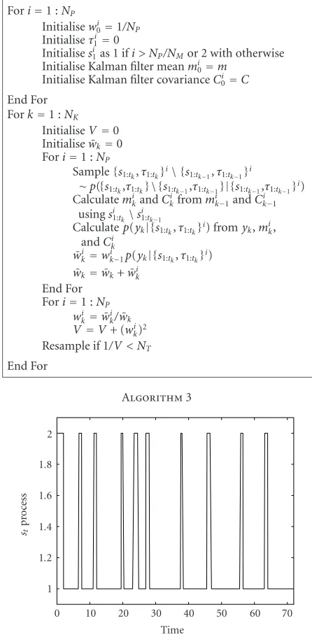
WithNPparticles andNKiterations, the algorithm is im-plemented as inAlgorithm 3.

The true trajectory through the discrete space is given in Figure 3. The hypothesis for the trajectory through the dis-crete space for some of the particles is shown in Figure 4. Note that, as a result of the resampling, all the particles have the same hypothesis for the majority of the trajectory through the discrete space, which is well matched (for the

Fori=1 :NP

Initialise Kalman filter meanmi

0=m

Initialise Kalman filter covarianceCi

0=C

End For Fork=1 :NK

InitialiseV=0 Initialise ¯wk=0

Figure3: True trajectory for target throughststate space.

most part) to the true trajectory. The diversity of the parti-cles represents the uncertainty over the later part of the state sequence with the particles representing different hypothe-sised times and numbers of recent regime switches.

6.3. Classification on the basis of manoeuvrability The proposals that are well suited to each class each use the associated class’ prior as their proposal:

qs1:tk,τ1:tk \

0 10 20 30 40 50 60 70

Figure4: A subset of the particles’ hypothesised trajectories throughstspace. (a) Particle 1. (b) Particle 2. (c) Particle 3. (d) Particle 4. (e) Particle 5. (f) Particle 6. (g) Particle 7. (h) Particle 8. (i) Particle 9.

¯

Having processed thekmeasurement, theith particle in the jth stratum stores the time of the hypothesised last

0 40 80 120 160 200 Time

0 0.2 0.4 0.6 0.8 1

st

d

·

(

p

(class))

1 2 3

(a)

0 40 80 120 160 200

Time 0

0.2 0.4 0.6 0.8 1

st

d

·

(

p

(class))

1 2 3

(b)

0 40 80 120 160 200

Time 0

0.2 0.4 0.6 0.8 1

st

d

·

(

p

(class))

1 2 3

(c)

Figure5: Standard deviation (std) of estimated classification probabilities, (p(class)), across ten filter runs for simulations according to each of the three models, labelled as 1, 2, and 3. (a) Data simulated from class 1. (b) Data simulated from class 2. (c) Data simulated from class 3.

Each stratum also storesw_k(j). The reader is referred to the preceding sections’ summaries of the algorithms for the im-plementation details.

NP=25 particles are used per stratum, each is initialised as described previously with a uniform distribution over the classes and with the weights on the strata initialised as be-ing equal. Resamplbe-ing for a given stratum takes place if the approximate effective sample size given in (11) for the stra-tum falls belowNT =12.5. Since each of theNM =3 strata has NP = 25 particles, the computational cost is approx-imately that of a multiple hypothesis tracker which main-tains 75 hypotheses; the algorithm is practicable in terms of its computational expense.

However, it should be noted that, for this difficult prob-lem of joint tracking and classification using very similar models, the number of particles used is small. This is inten-tional and is motivated by the need to look at the difference

between the variance in the class membership probabilities and the variance of the strata weights.

0 40 80 120 160 200 Time

0 0.2 0.4 0.6 0.8 1

st

d

·

(

w

(class))

1 2 3

(a)

0 40 80 120 160 200

Time 0

0.2 0.4 0.6 0.8 1

st

d

·

(

w

(class))

1 2 3

(b)

0 40 80 120 160 200

Time 0

0.2 0.4 0.6 0.8 1

st

d

·

(

w

(class))

1 2 3

(c)

Figure6: Variance of strata weights across ten filter runs for simulations according to each of the three models. (a) Data simulated from class 1. (b) Data simulated from class 2. (c) Data simulated from class 3.

calculating the probabilities of all the classes for every sam-ple.

It is difficult to draw many conclusions from the varia-tions across the true class. Since such issues are quite spe-cific to the models and parameters, which are not the fo-cus of this paper, this is not further investigated or dis-cussed.

7. CONCLUSIONS

Particle filtering has been applied to the use of semi-Markov models for tracking manoeuvring targets. An architecture has been proposed that enables particle filters to be both ro-bust and efficient when classifying targets on the basis of their dynamic behaviour. It has been demonstrated that it is pos-sible to jointly track such manoeuvring targets and classify their manoeuvrability.

ACKNOWLEDGMENTS

This work was funded by the UK MoD Corporate Research Programme. The author also gratefully acknowledges the award of his Industrial Fellowship by the Royal Commis-sion for the Exhibition of 1851. The author would like to thank John Boyd and Dave Sworder for useful discussions on the subject of joint tracking and classification associated with the use of semi-Markov models and Arnaud Doucet and Matthew Orton for discussions of how particle filters can be used in such problems. The author also thanks the reviewers for their comments.

REFERENCES

[1] D. R. Cox and V. Isham, Point Processes, Chapman and Hall, New York, NY, USA, 1980.

switching,” IEEE Trans. Automatic Control, vol. 36, no. 2, pp. 238–243, 1991.

[3] D. D. Sworder, M. Kent, R. Vojak, and R. G. Hutchins,

“Re-newal models for maneuvering targets,” IEEE Trans. on

Aerospace and Electronics Systems, vol. 31, no. 1, pp. 138–150, 1995.

[4] N. J. Gordon, S. Maskell, and T. Kirubarajan, “Efficient par-ticle filters for joint tracking and classification,” inSignal and Data Processing of Small Targets, vol. 4728 ofProceedings SPIE, pp. 439–449, Orlando, Fla, USA, April 2002.

[5] S. Challa and G. Pulford, “Joint target tracking and classifica-tion using radar and ESM sensors,”IEEE Trans. on Aerospace and Electronics Systems, vol. 37, no. 3, pp. 1039–1055, 2001. [6] Y. Boers and H. Driessen, “Integrated tracking and

classifica-tion: an application of hybrid state estimation,” inSignal and Data Processing of Small Targets, vol. 4473 ofProceedings SPIE, pp. 198–209, San Diego, Calif, USA, July 2001.

[7] S. Herman and P. Moulin, “A particle filtering approach to FM-band passive radar tracking and automatic target recog-nition,” inProc. IEEE Aerospace Conference, vol. 4, pp. 1789– 1808, BigSky, Mont, USA, March 2002.

[8] M. S. Arulampalam, S. Maskell, N. J. Gordon, and T. Clapp, “A tutorial on particle filters for online nonlinear/non-Gaussian Bayesian tracking,” IEEE Trans. Signal Processing, vol. 50, no. 2, pp. 174–188, 2002.

[9] J. Vermaak, S. J. Godsill, and A. Doucet, “Radial basis function regression using trans-dimensional sequential Monte Carlo,” inProc. 12th IEEE Workshop on Statistical Signal Processing, pp. 525–528, St. Louis, Mo, USA, October 2003.

[10] A. Doucet, J. F. G. de Freitas, and N. J. Gordon, Eds., Sequen-tial Monte Carlo Methods in Practice, Springer, New York, NY, USA, 2001.

[11] F. Le Gland and N. Oudjane, “Stability and uniform

ap-proximation of nonlinear filters using the Hilbert metric, and application to particle filters,” Tech. Rep. RR-4215, INRIA, Chesnay Cedex France, 2001.

[12] D. Crisan and A. Doucet, “Convergence of sequential Monte Carlo methods,” Tech. Rep. CUED/F-INFENG/TR381, De-partment of Engineering, University of Cambridge, Cam-bridge, UK, 2000.

[13] P. M. Baggenstoss, “The PDF projection theorem and the class-specific method,” IEEE Trans. Signal Processing, vol. 51, no. 3, pp. 672–685, 2003.

[14] Y. Bar-Shalom and X. R. Li,Multitarget-Multisensor Tracking: Principles and Techniques, YBS Publishing, Storrs, Conn, USA, 1995.

Simon Maskellis a Ph.D. degree graduand and holds a first-class degree with Distinc-tion from Department of Engineering, Uni-versity of Cambridge. His Ph.D. degree was funded by one of six prestigious Royal Com-mission for the Exhibition of 1851 Indus-trial Fellowships awarded on the basis of outstanding excellence to researchers work-ing in British industry. At QinetiQ, he is a Lead Researcher for tracking in the