FULL PAPER
Source rupture process of the 2018
Hokkaido Eastern Iburi earthquake deduced
from strong-motion data considering seismic
wave propagation in three-dimensional velocity
structure
Kimiyuki Asano
*and Tomotaka Iwata
Abstract
The source rupture process of the 2018 Hokkaido Eastern Iburi earthquake (MJMA 6.7) was analyzed by a kinematic waveform inversion method using strong-motion data in 0.04–0.5 Hz. This earthquake occurred close to the Hidaka Collision Zone and the Ishikari depression, where the crustal structure is rather complex. Thus, we used a three-dimen-sional velocity structure model to compute the theoretical Green’s functions by the finite difference method. A source fault model with strike-angle variation was set based on the spatial distribution of the early aftershocks. The strong-motion stations used for the source inversion were selected based on the result of forward ground strong-motion simula-tion of a moderate aftershock. The slip in the first 5 s was relatively small, but an area of significant slip with peak slip of 1.7 m was found in the depth range from 22 to 32 km. The rupture propagated upward mainly in the southwest direction. Based on the regional crustal structure and the configuration of the Moho discontinuity, the large-slip area was thought to be located in the lower crust, and its rupture did not reach the upper part of the continental crust. Most of the early aftershocks occurred around the large-slip area. The later aftershocks at the depth shallower than 20 km occurred outside the causative source fault of the mainshock. Three-dimensional ground motion simulation demonstrated that the heterogeneous source process and the three-dimensional basin and crustal velocity structure brought a large velocity pulse to an area to the southwest of the source fault, where the largest PGV was observed during the mainshock. The spatial distribution of the simulated PGV resembled the observed PGV distribution except some sites located inside the Ishikari depression where thick Quaternary soft low-velocity sediments exist at the top of the basin.
Keywords: The 2018 Hokkaido Eastern Iburi earthquake, Source rupture process, Kinematic source inversion, Strong-motion data, Three-dimensional velocity structure, Ground Strong-motion simulation
© The Author(s) 2019. This article is distributed under the terms of the Creative Commons Attribution 4.0 International License (http://creat iveco mmons .org/licen ses/by/4.0/), which permits unrestricted use, distribution, and reproduction in any medium, provided you give appropriate credit to the original author(s) and the source, provide a link to the Creative Commons license, and indicate if changes were made.
Introduction
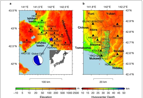
Hokkaido Island was rocked by an MJMA 6.7 earthquake, called the 2018 Hokkaido Eastern Iburi earthquake. It occurred to the west of the Hidaka Collision Zone, Cen-tral Hokkaido, Japan, at a depth of 37 km, at 03:08 JST on September 6, 2018 (18:08 UTC on September 5, 2018)
(Fig. 1). This earthquake drew significant attentions to a number of landslides in the epicentral region (Yamagishi and Yamazaki 2018; Yamaguchi et al. 2019), liquefaction in residential areas in Sapporo and other cities (Hirose et al. 2018; Karimzadeh and Matsuoka 2018; Kuwahara et al. 2018), and blackout in the whole Hokkaido Island (Ozaki et al. 2019). An overview of casualties, damages and government responses was reported by Takahashi and Kimura (2019).
Open Access
*Correspondence: [email protected]
The hypocenter of the 2018 Hokkaido Eastern Iburi earthquake is located by the Japan Meteorological Agency (JMA) beneath the western part of the Hidaka Collision Zone, which is an arc–arc collision system in Hokkaido Island. The Kuril forearc sliver moved south-westward since the Late Miocene and collided with the Northeast Japan Arc due to the oblique subduction of the Pacific plate (Kimura 1986). This tectonic setting makes the high-velocity Hidaka body thrust steeply over the low-velocity crust of the Northeast Japan Arc at the western edge of the Kuril forearc (Arita et al. 1998; Iwasaki et al. 2004; Kita et al. 2012; Moriya et al. 1998). Mature continental-type crust of the Kuril Arc has been exposed in the Hidaka Mountains as a result of collision (Kimura 1996). The collision of the Kuril forearc sliver is also developing the foreland fold-and-thrust belt with very thick sedimentary basins to the west of the Hidaka Mountains. The westernmost part of this belt is called the Ishikari depression (Ishikari Lowland) (Iwasaki et al.
2004; Kimura 1996). Accordingly, the crustal struc-ture in this region is rather complex due to the above-mentioned situation. Recently, Kita et al. (2012) imaged P- and S-wave velocity structure by a travel-time tomog-raphy technique and concluded that the arc–arc colli-sion of this region produced M7-class earthquakes at anomalously deep depths at sharp material boundaries between uppermost mantle and crustal materials (MJMA 6.7 Hidaka earthquake at 55 km on January 21, 1970 and
MJMA 7.1 Urakawa-oki earthquake at 40 km on March 21, 1982). The 2018 Hokkaido Eastern Iburi earthquake could be thought to be one of such anomalously deep earthquakes in the Hidaka Collision Zone.
The strong ground motions during this event were observed by nation-wide and regional strong-motion networks. We have collected strong-motion data from K-NET, KiK-net, and F-net of the National Research Institute for Earth Science and Disaster Resilience (NIED) (Aoi et al. 2011; National Research Institute for
141°E 141.5°E 142°E 142.5°E
42°N
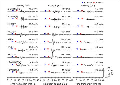
Earth Science and Disaster Resilience 2019a, b; Okada et al. 2004), and seismic intensity observation networks operated by JMA, Hokkaido Government, and City of Sapporo (Nishimae 2004). The observed PGA exceeded 1500 cm/s2 at KiK-net IBUH01 and K-NET HKD127 both located in Oiwake of Abira town, Yufutsu District, Iburi Subprefecture. The site is in Yuni-Abira Lowlands, which is a narrow valley, the eastern part of the Ishikari depression. The observed PGV exceeded 100 cm/s at several strong-motion stations in Mukawa, Atsuma, and Abira towns. The largest one among the collected data was the record at station HKD126 in Mukawa, which is a coastal town known for Shishamo fish, in the east of the Yufutsu basin. Seismic intensity of 7 in JMA scale was recorded during this event at one JMA seismic intensity station (station code 41407 in Atsuma town). Figure 2 shows velocity waveforms observed at strong-motion stations in the vicinity of the epicenter. These velocity waveforms were processed by integrating the original acceleration waveform data observed at those stations,
and bandpass-filtered in the frequency range from 0.05 to 20 Hz. Manually picked onset times of P- and S-waves are indicated by blue and red triangles in this figure. The observed records clearly show difference in arrival time between the initial S-wave onset and the largest ampli-tude (Fig. 2 and Additional file 1: Fig. S1). The fact indi-cates the possibility that the initial part of the source fault rupture was weak and significant slips generating strong ground motions occurred shortly afterward. The arrival time of the largest amplitude is the earliest at station 47004, which implies that seismic source generating this pulse is relatively close to this station.
The spatial PGA and PGV distributions show larger amplitude to the west of the source region, particularly in the Yufutsu and Ishikari basins, both are part of the Ishi-kari depression. The large amplification of long-period ground motions in the Yufutsu sedimentary basin was also observed during the 2003 Tokachi-oki earthquake (MW 8.3) causing severe damages to large oil storage tanks in Tomakomai by liquid sloshing (Aoi et al. 2008;
Velocity (NS) Velocity (EW) Velocity (UD)
P−wave S−wave
IBUH01(D)x5 15.0 cm/s 14.0 cm/s 5.6 cm/s
IBUH01(S) 105.0 cm/s 98.3 cm/s 38.1 cm/s
HKD127 57.6 cm/s 85.0 cm/s 43.6 cm/s
HKD128 69.5 cm/s 108.6 cm/s 26.9 cm/s
51200 46.4 cm/s 117.9 cm/s 22.3 cm/s
47004 67.5 cm/s 136.4 cm/s 15.7 cm/s
HKD126 48.8 cm/s 151.1 cm/s 13.7 cm/s
HDKH04(D)x5 14.4 cm/s 21.5 cm/s 5.8 cm/s
HDKH04(S) 48.1 cm/s 44.8 cm/s 9.9 cm/s
0 5 10 15 20 25 30 35 40 Time from origin time (s)
0 5 10 15 20 25 30 35 40 Time from origin time (s)
−160−80 0 80 160
cm/s
0 5 10 15 20 25 30 35 40 Time from origin time (s)
Hatayama et al. 2007; Koketsu et al. 2005; Maeda and Sasatani 2004). The Ishikari depression including the Ishikari and Yufutsu sedimentary basins has exception-ally thick Quaternary to Paleogene sediments, whose depth to the Early Cretaceous bedrock is around 8 km (Aoi et al. 2008; Yokokura et al. 2014). Thus, the effects of the three-dimensional sedimentary and crustal structure on the seismic waves need to be considered while study-ing the source rupture process usstudy-ing regional strong-motion data.
In this paper, the source rupture process of the 2018 Hokkaido Eastern Iburi earthquake is deduced from strong-motion data by a kinematic waveform inversion method. Because of the above-mentioned reasons, we also considered a three-dimensional velocity structure model in the source inversion analysis. The obtained source rupture process will be discussed with respect to the crustal structure and the spatiotemporal aftershock distribution. Then, a three-dimensional ground motion simulation demonstrates spatial distribution of ground motions focusing attention on the effects of the heteroge-neous source rupture process and the three-dimensional underground velocity structure.
Finite source inversion method and source fault model setting
The kinematic source rupture process of this earth-quake was analyzed by the multiple time-window linear waveform inversion method developed by Hartzell and Heaton (1983) and Olson and Apsel (1982). The observa-tional equation of this problem is based on the represen-tation theorem (Maruyama 1963; Burridge and Knopoff 1964). The same technique has been widely applied to strong-motion data for many past large earthquakes (e.g., Asano and Iwata 2016; Ma et al. 2001; Sekiguchi et al. 2000; Suzuki et al. 2011; Wald and Heaton 1994; Yoshida et al. 1996). Our source inversion code has been tested in the Source Inversion Validation project (Gallovič and Ampuero 2015; Mai et al. 2016).
A source fault model was assumed by referring to the spatial distribution of the early aftershocks in the JMA unified hypocenter catalog, which is presented in Fig. 3. The aftershocks occurring within 2 h from the main-shock’s origin time were plotted in this figure. Most of the aftershocks in this time-period occurred at the depth deeper than 30 km. The early aftershock distribu-tion shows clearly a steep fault plane dipping eastward. The strike angle of the source fault changes along the strike direction like a byobu (Japanese folding screen with two or more panels). Thus, we assumed a source model which consists of three fault planes by changing strike angle. The dip angle is assumed to be 70° referring to the
aftershock distribution and the centroid–moment ten-sor solution of Global CMT Project (Ekström et al. 2012). The assumed source fault model is also plotted in Fig. 3.
The fault plane model was divided into small equal-area subfaults (3 km × 3 km). The temporal moment-release history at the center of each subfault was represented by several time-windows. The unknown model parameters in this source inversion analysis were the amplitude of the basis functions corresponding to each time-window at each subfault. The number of the time-windows at each subfault was set at 4 after preliminary analysis. The rupture front of the first time-window propagated radi-ally at a constant velocity from the rupture starting point fixed at the hypocenter, and we assumed that the rupture propagates continuously beyond the segment bound-ary. Since each time-window at each subfault has two orthogonal rake angles to represent variable rake angle, the total number of the unknown model parameters was 80 × 4 × 2 = 640. The rake angle variation was lim-ited within a certain range, as described in Table 1. The problem could be solved using the linear least-squares method with a nonnegative constraint (Lawson and Han-son 1974). A spatiotemporal smoothing constraint was included following Sekiguchi et al. (2000) to stabilize the solution. A relative weight of the smoothing constraint equation against the observational equation and the rupture propagation velocity triggering the first time-window were determined so as to minimize the Akaike’s Bayesian information criterion (ABIC) (Akaike 1980).
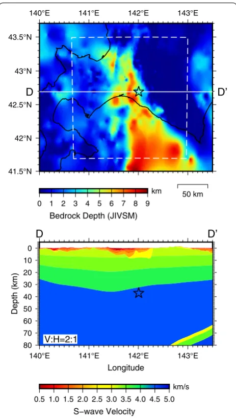
In this study, the theoretical Green’s functions were computed by the three-dimensional finite differ-ence method (FDM) using a three-dimensional veloc-ity structure model, the Japan Integrated Velocveloc-ity Structure Model Version 1 (JIVSM; Koketsu et al. 2012). This velocity structure model is represented by a stack
of isotropic homogeneous layers from near-surface sedi-mentary layers to subducting oceanic plates, and each of the layer boundaries was modeled by integrating many kinds of geophysical exploration data and seismic wave modeling (Koketsu et al. 2012). Figure 4 shows the bed-rock (VS= 2.9 km/s) depth distribution and a west–east 141.8°E
141.8°E
142°E 142°E
142.2°E 142.2°E
42.5°N 42.6°N 42.7°N 42.8°N 42.9°N
C
C’
B
B’
A
A’
M
JMA1 2 3 4 5 6
0
10
20
30
40
50
Depth (km
)
’
0
10
20
30
40
50
Depth (km
)
’
0
10
20
30
40
50
Depth (km)
−20 −10 0 10 20
Distance (km)
C
C
B
B
A
A’
JMA unified hypocenter catalog MJMA≥ 1.0 (N = 149) 2018/09/06 03:07−05:07 (JST)
cross-section of JIVSM. The model reflects lateral vari-ation produced by the Hidaka Collision Zone and the foreland fold-and-thrust belt. Area to the west and south of the epicenter has relatively thick Quaternary to Paleogene sediments. The lowest S-wave velocity of the above-mentioned model is 0.6 km/s in the area shown in the map. That is, Holocene and Upper Pleistocene layers which may have S-wave velocity lower than 0.6 km/s are not included in the present velocity model for this area.
A staggered-grid FDM code, which has been coded and used in Asano et al. (2016), was used to compute the Green’s functions. This code solves the elastody-namic wave equation in a velocity–stress formulation with fourth-order accuracy in space and second-order accuracy in time. The FDM model space, occupying an area of 190 km (E–W) × 200 km (N–S) in southern and central Hokkaido corresponding to the geographical area shown in Fig. 4, extends to a depth of 80 km below the ground surface. The model was discretized using a uniform grid of 0.1 km along the horizontal and verti-cal axes. The total number of the grid points was 1901 × 2001 × 802 = 3,050,728,602. The boundary condition between the isotropic homogeneous layers was intro-duced by adopting the technique of Moczo et al. (2002). A zero-stress formulation was introduced for the free surface boundary condition at the top of the model space (e.g., Levander 1988; Graves 1996). A multi-axial perfectly matched layer (PML) was applied to the model boundaries, except for the free surface, to avoid non-physical reflections (Meza-Fajardo and Papageor-giou 2008; Zeng et al. 2011). The grid thickness of the PML domain was set at 10 grids. Anelastic attenuation
in the medium was included in the form of a linear fre-quency-dependent Q operator Q(f) =Q0(f/f0) following the method proposed by Graves (1996). The reference frequency f0 is set at 0.5 Hz. The three-dimensional wave propagation was simulated for 80 s after the ori-gin time at increments of 0.005 s, which made the total number of time steps in a simulation be 16,000.
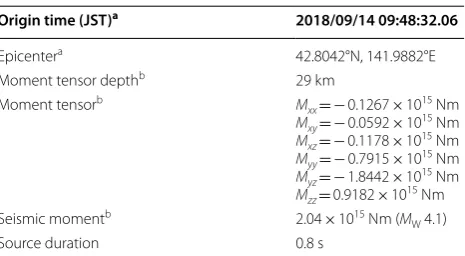
To choose strong-motion stations for the source inversion analysis, we first simulate ground motions for an MW 4.1 aftershock, which occurred at 9:48 on
Table 1 Summary of fault model setting in waveform inversion analysis
a The origin time and hypocenter were taken from the JMA unified earthquake
catalog
Origin time (JST)a 2018/09/06 03:07:59.33
Hypocentera 42.6908°N, 142.0067°E, 37.04 km
Fault segment South Central North
Strike/dip 10°/70° 355°/70° 5°/70° Rake angle variation 90° ± 45° 90° ± 45° 90° ± 45°
Length 12 km 9 km 9 km
Width 24 km 24 km 24 km
Top depth 18.7 km 18.7 km 18.7 km Bottom depth 41.3 km 41.3 km 41.3 km Subfault size 3 km × 3 km
Number of subfaults 32 24 24 Number of time-windows 4
Duration/time-shift of time-window 2.0 s/1.0 s
140°E 141°E 142°E 143°E
41.5°N 42°N 42.5°N 43°N 43.5°N
50 km 0 1 2 3 4 5 6 7 8 9
Bedrock Depth (JIVSM)
km
’
0 10 20 30 40 50 60 70 80
Depth (k
m
)
140°E 141°E 142°E 143°E
Longitude
D D
D
D ’
V:H=2:1
0.5 1.0 1.5 2.0 2.5 3.0 3.5 4.0 4.5 5.0
S−wave Velocity
km/s
September 14, 2018 (JST). The epicenter location of this aftershock was given referring to the JMA uni-fied hypocenter catalog. A point source moment ten-sor was assumed for as the source term, and we used the moment tensor solution of F-net, NIED. The source parameters of this aftershock are summa-rized in Table 2. At the KiK-net stations (station code of IBUHxx, HDKHxx, IKRHxx, SRCHxx), observed records from downhole sensors, were used for this analysis to avoid effects of very soft sediments. The broadband sensors of F-net were installed in an obser-vational tunnel at each station (HID and HSS), and the strong-motion sensors of the K-NET stations (HKDxxx) were installed on the ground surface. The original acceleration records were numerically inte-grated in the time domain to obtain the velocity records except the F-net stations being equipped with a veloc-ity-type strong-motion seismograph. Some near-source strong-motion stations to the west of the epicenter such as HKD126, HKD128, 47004, and 51200 were excluded in the source inversion analysis because those ground motion records were strongly affected by the nonlinear effects of the near-surface soil material dur-ing extremely strong shakdur-ing (e.g., Dhakal et al. 2019; Ikeda and Takagi 2019; Takai et al. 2019).
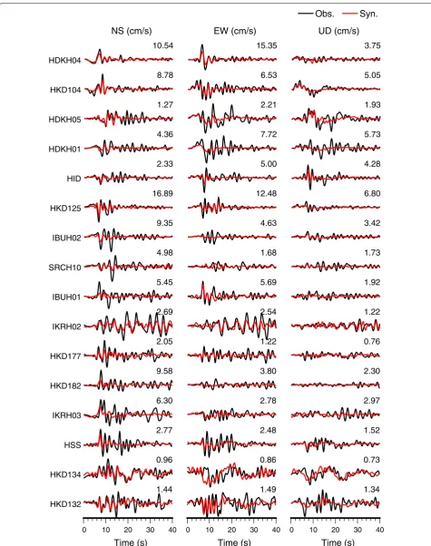
After inspecting waveform fitting at strong-motion sta-tions in central and southern Hokkaido, we finally chose 16 strong-motion stations of K-NET, KiK-net and F-net shown by the solid triangles in Fig. 1a. The comparison between the observed and simulated velocity waveforms at those strong-motion stations is presented in Additional file 2: Fig. S2. The simulated waveforms using the three-dimensional velocity structure model for the selected stations (Additional file 2: Fig. S2) are better than the simulated waveforms using the one-dimensional velocity
structure model (Additional file 3: Fig. S3) particularly in terms of elongation of the ground motion duration by the three-dimensional effects. Those 1D synthetics were cal-culated by the discrete wavenumber method (Bouchon 1981) with the reflection and transmission matrix (Ken-nett and Kerry 1979), and the one-dimensional veloc-ity structure model for each station is constructed by extracting the one-dimensional profiles beneath the site from JIVSM. Thus, the near-surface response was com-mon between 1D and 3D modeling. If we use an identi-cal one-dimensional velocity model for all the stations, waveform fitting would become much worse than Addi-tional file 3: Fig. S3.
Then, the Green’s functions for the source inversion of the mainshock were computed by FDM. Since each sub-fault must have two orthogonal slip components (90° and 0°), the total number of the required computing runs was 160. Both observed velocity waveforms and synthetic Green’s functions were bandpass-filtered from 0.04 to 0.5 Hz, and then resampled at 5 Hz. Forty-second length of the velocity waveform starting from 1 s before the initial S-wave arrival was used for the source inversion analysis. The initial S-wave arrival of both observed and synthetic waveforms was picked up carefully by visual inspection to make the timing of the S-wave onset same among the waveforms and to compensate the residual between the observed and theoretical travel times. Exam-ples of the manual picking for the observed waveforms are demonstrated in Additional file 1: Fig. S1.
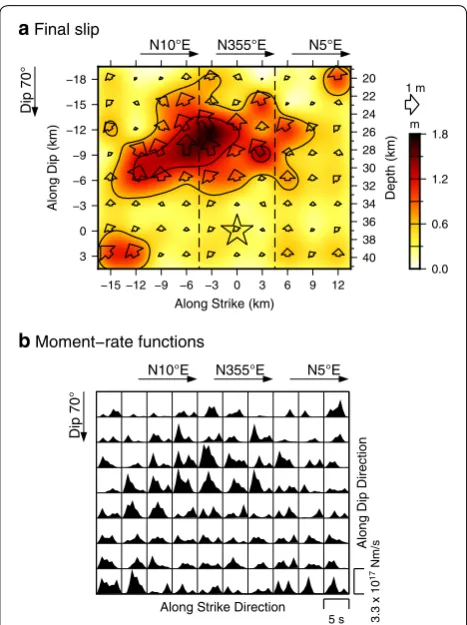
Results
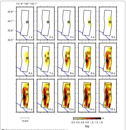
Figure 5 shows the estimated final slip distribution. This source model has a seismic moment of 1.99 × 10¹⁹ Nm (MW 6.8). The synthetic waveforms explain character-istics of the observed waveforms fairly well (Fig. 6). The snapshot at every 1 s was plotted as map view in Fig. 7. The slip in the first 5 s was small; then, the rupture propa-gated upward in the southwest direction. The rupture also spread to the north afterward. The entire rupture finished within 15 s. The best estimate for the propaga-tion velocity triggering the rupture front of the first time-window was 1.8 km/s. The peak slip reaching 1.7 m was found at a depth of about 26 km, southwest of the epi-center. The average slip over the source fault was 0.59 m. The slip-weighted average rake angle over the entire fault was 103°, which was similar to the published moment tensor solutions by the Global CMT project (strike 349°, dip 68°, rake 102°) and NIED F-net (strike 349°, dip 65°, rake 107°). There were relatively large slips at the south-bottom edge of the assumed source fault. Generally, it is not easy to judge whether such a large slip near the edge of the assumed source fault is true slip or artifact.
Table 2 Summary of source parameters in the aftershock waveform modeling
a The origin time and hypocenter were taken from the JMA unified earthquake
catalog
b The moment tensor solution was taken from the NIED F-net moment tensor
catalog (National Research Institute for Earth Science and Disaster Resilience
2019b)
Origin time (JST)a 2018/09/14 09:48:32.06
Epicentera 42.8042°N, 141.9882°E Moment tensor depthb 29 km
But, the contribution of that slip to the waveforms is not significant.
Significant slip larger than 1 m was estimated in the depth range from 22 to 32 km. Hereafter, we call it large-slip area. The Moho depth around the epicenter in JIVSM is approximately 32 km. Matsubara et al. (2017) also pub-lished a digital map of the Moho discontinuity beneath the Japanese Islands derived from three-dimensional seis-mic tomography. In their model, the depth of the Moho discontinuity in the source region of the 2018 Hokkaido Eastern Iburi earthquake is also 32–34 km, and it slants gradually down to the south. Besides, the hypocenter is close to the profile A in Fig. 6 of Kita et al. (2012), and their model also imaged the Moho discontinuity at depth around 32–34 km. The fault rupture stopped at a depth of about 20 km, which was deeper than the upper and lower crust boundary. Therefore, the rupture of the 2018 Hokkaido Eastern Iburi earthquake initiated at nearly top of the upper mantle, and the small slips in the first
5 s correspond to the early stage of the rupture occur-ring below the Moho discontinuity. Then, the large slip occurred in the depth range from 32 to 22 km within the lower crust. These temporal rupture characteristics were quite consistent with the characteristics of the observed waveforms in the near-source region as mentioned in the introduction. In this regard, this earthquake is different from most Japanese crustal earthquakes, which usually occur in the upper crust.
The 1982 Urakawa-oki earthquake (MJMA 7.1, MW 6.9) occurred at 42.07°N, 142.60°E at a depth of 40 km on the deep extension of one of thrust faults belonging to the Ishikari Lowland Eastern Edge Fault System (Kita et al. 2012). The source fault of the 1982 Urakawa-oki earth-quake was a thrust fault dipping to northeast (Suetsugu and Nakanishi 1988). The geometry and depth range of the source fault of the 2018 Hokkaido Eastern Iburi earthquake were similar to that of the 1982 Urakawa-oki earthquake. Both of the earthquakes are thrust events in the lower crust under the common tectonic condition controlled by the regional stress filed of the Hidaka Col-lision Zone.
Discussions
Slip distribution of the mainshock and temporal aftershock distribution
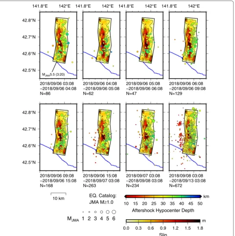
The temporal aftershock distribution was compared with the final slip distribution (Fig. 8). The aftershock locations were taken from the JMA unified hypocenter catalog. Eight periods are shown in this figure. The loca-tion of the largest aftershock (MJMA 5.5), which occurred 12 min after the mainshock, was nearly southern edge of the source fault of the mainshock. It suggests a possibil-ity that this largest aftershock was induced by the stress accumulation due to the rupture of the large-slip area during the mainshock. Most of the aftershocks occurring in the first 6 h were located surrounding the large-slip area, particularly in the deeper part of the mainshock’s source fault. Then, the aftershock activity in the depth shallower than 20 km becomes active. This temporal aftershock distribution also supports that the rupture of the mainshock did not reach the upper part of the crust, which is shallower than 20 km.
We have referred to the JMA unified hypocenter catalog, which is a homogeneous earthquake catalog covering the whole territory of Japan. A single one-dimensional velocity model was used for the inland earthquakes in the JMA catalog. Thus, the theoretical travel time calculated from the JMA velocity model may be different from the theoretical travel time cal-culated for each station from JIVSM. Generally, those theoretical travel times may not perfectly correspond
20
Time (s) Time (s)
0 10 20 30 40 0 10 20 30 40 0 10 20 30 40
Time (s)
HKD132
1.44 1.49 1.34
HKD134
0.96 0.86 0.73
HSS
2.77 2.48 1.52
IKRH03
6.30 2.78 2.97
HKD182
9.58 3.80 2.30
HKD177
2.05 1.22 0.76
IKRH02
2.69 2.54 1.22
IBUH01
5.45 5.69 1.92
SRCH10
4.98 1.68 1.73
IBUH02
9.35 4.63 3.42
HKD125
16.89 12.48 6.80
HID
2.33 5.00 4.28
HDKH01
4.36 7.72 5.73
HDKH05
1.27 2.21 1.93
HKD104
8.78 6.53 5.05
HDKH04
10.54 15.35 3.75
NS (cm/s) EW (cm/s) UD (cm/s) Obs. Syn.
to the observed travel time because of the local site effects and the Earth’s heterogeneities as seen in Addi-tional file 2: Fig. S2. The initial S-wave arrival of both observed and synthetic waveforms were picked up carefully by visual inspection to compensate the resid-ual between the observed and theoretical travel times in our source inversion analysis. Therefore, the differ-ence in the assumed velocity structure model will not
apparently affect the slip distribution because the spa-tiotemporal slip was solved relative to the hypocenter location and the origin time. Nevertheless, the appli-cation of the local velocity structure model makes us improve the reproductivity of waveforms itself and see more precise image of the source process (e.g. Asano and Iwata 2011).
Spatial distribution of ground motions during the mainshock
A forward ground motion simulation using FDM for the mainshock was carried out to demonstrate effects of the heterogeneous source rupture process and the three-dimensional velocity structure on the strong ground motions in central and southern Hokkaido. The geo-graphical area for the FDM simulation (190 km × 200 km)
is same as the computations of Green’s functions described before (Fig. 4). The kinematic source model obtained in this study was used for this FDM simulation. The output ground motions were obtained at the free surface (top of VS= 600 m/s layer in this model).
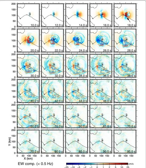
Figure 9 presents snapshots of the ground velocities in the EW component. The same figures for the NS and UD components are presented in Additional file 4: Fig. S4 and
141.8°E 142°E
42.5°N 42.6°N 42.7°N 42.8°N
MJMA5.5 (3:20)
2018/09/06 03:08 −2018/09/06 04:08 N=86
141.8°E 142°E
2018/09/06 04:08 −2018/09/06 05:08 N=62
141.8°E 142°E
2018/09/06 05:08 −2018/09/06 06:08 N=47
141.8°E 142°E
2018/09/06 06:08 −2018/09/06 09:08 N=129
42.5°N 42.6°N 42.7°N 42.8°N
10 km 2018/09/06 09:08 −2018/09/06 15:08 N=168
2018/09/06 15:08 −2018/09/07 03:08 N=263
2018/09/07 03:08 −2018/09/08 03:08 N=234
2018/09/08 03:08 −2018/09/13 03:08 N=672
EQ. Catalog: JMA M≥1.0
MJMA 1 2 3 4 5 6
10 15 20 25 30 35 40 45 50
Aftershock Hypocenter Depth
km
0.0 0.3 0.6 0.9 1.2 1.5 1.8
Slip
m
0 50 100 150 200
0 50 100 150 200
10.0 s 12.0 s 14.0 s 16.0 s 18.0 s
0 50 100 150 200
0 50 100 150 200
20.0 s 22.0 s 24.0 s 26.0 s 28.0 s
0 50 100 150 200
0 50 100 150 200
30.0 s 32.0 s 34.0 s 36.0 s 38.0 s
0 50 100 150 200
0 50 100 150 200
40.0 s 42.0 s 44.0 s 46.0 s 48.0 s
0 50 100 150 200
0 50 100 150 200
50.0 s 55.0 s 60.0 s 65.0 s 70.0 s
0 50 100 150 200
Y (km)
0 50 100 150
X (km)
EW comp. (< 0.5 Hz)
050 100 150 200
Y (km)
0 50 100 150
X (km) 75.0 s
0 50 100 150 0 50 100 150
80.0 s
0 50 100 150 0 50 100 150 85.0 s
0 50 100 150 0 50 100 150 90.0 s
0 50 100 150 0 50 100 150 95.0 s
−25 −10 −5 −2 −1 0 1 2 5 10 25 cm/s
Additional file 5: Fig. S5, respectively. The geographical area of those maps corresponds to the FDM model space, which is represented by the broken rectangle in Fig. 4. At about 18 s after the origin time, a large amplitude velocity pulse (~ 20 cm/s), which is indicated by the black arrow in Fig. 9, hits the area to the southwest of the source fault, where large PGV was observed in Mukawa and Atsuma towns. This velocity pulse dominated in the EW compo-nent (Fig. 10). It was originated from the large-slip area, and it was amplified by the deep sedimentary layers in this area. But, the actual observed ground velocities at Mukawa (HKD126) and Atsuma (47004) (Fig. 2) were much larger than the simulated ground motions. It might be because that the present velocity structure model in this FDM simulation does not include near-surface Qua-ternary soft sedimentary layers, whose S-wave velocity is much lower than 0.6 km/s, as low as 0.1 km/s expected from the K-NET PS-logging information at HKD126 (National Research Institute for Earth Science and Disas-ter Resilience 2019a).
Since the ground motions were simulated at the top of engineering bedrock (VS = 0.6 km/s), the simulated ground motions could be interpreted as input motions at the bottom of shallow low-velocity layers. Existence of significant amplification by the shallow low-velocity lay-ers is also evidenced by the amplitude difference in the observed ground motions at uphole and downhole sen-sors of IBUH01 plotted in Fig. 2.
Duration of ground motions was long in the Ishikari and Yuftusu basins, and the wave propagation inside those basins looks slow compared to the other directions (Fig. 9). Figure 11 compares the simulated PGV with the observed PGV in the frequency range lower than 0.5 Hz. The spatial pattern of the simulated PGV distribution resembles the observed PGV map except the sites located inside the Ishikari depression, where existence of thick Late Pleistocene to Holocene low-velocity sediments is expected (e.g., Sagayama et al. 2017; Sato and Komat-subara 2014). This result supports that the source model obtained in this study is adequate to model the ground motions in this frequency range.
0
10
20
30
40
Time (s)
−15 −10 −5 0
5 10 15 20 25 30 35 40
Distance (km)
0 10 cm/s
E E’
Southwest Northeast
a Profile E−E’ EW comp.
0
10
20
30
40
Time (s)
−15 −10 −5 0
5 10 15 20 25 30 35 40
Distance (km)
0 10 cm/s
E E’
Southwest Northeast
b Profile E−E’ NS comp.
As a future issue on the ground motion modeling in this area, investigation and modeling of the shallow low-velocity layers would be required for quantitatively evalu-ating the surface ground motions in the area with thick Quaternary sediments. Moreover, this FDM simulation was limited up to 0.5 Hz. Thus, it is also necessary to model the broadband ground motions by including the effects of near-surface low-velocity sediments for evalu-ating quantitatively the input ground motions to build-ings and landslides in the disaster-affected area.
Conclusions
The source rupture process of the 2018 Hokkaido East-ern Iburi earthquake (MJMA 6.7) was estimated by the kinematic waveform inversion technique using strong-motion waveform data and three-dimensional veloc-ity structure model. The theoretical Green’s functions were computed using a three-dimensional velocity structure model JIVSM by FDM to include the effects of wave propagation controlled by complex crustal structures such as the Hidaka Collision Zone and the foreland fold-and-thrust belt in the study region. The source fault was dipping to eastward with variation in strike angle. The result of the kinematic source inver-sion revealed that the initial rupture in the first 5 s was weak, and then rupture propagated up- and south-westward. The peak slip reaching 1.7 m was found at a depth of approximately 26 km to the southwest of the hypocenter. The total seismic moment was estimated to be 1.99 × 10¹⁹ Nm (M
W 6.8). The large-slip area was
restricted in the depth range from 22 to 32 km, which is in the lower crust. Thus, the rupture of the 2018 Hok-kaido Eastern Iburi earthquake initiated at nearly top of the upper mantle, and propagated upward beyond the Moho discontinuity. The crustal structure might control such rupture characteristics of this earthquake as well as the 1982 Urakawa-oki earthquake (MW 6.9) occurring approximately 85 km southeast of the 2018 Hokkaido Eastern Iburi earthquake. More detailed works on the fault geometry and crustal structure may improve physical understanding of this earthquake and reproduction of the waveforms. The spatial extent of the causative source fault of the mainshock was also supported by the spatial and temporal distributions of aftershocks. The forward three-dimensional ground motion simulation demonstrated that the combination of heterogeneous source process and three-dimensional basin and crustal velocity structure brought a large velocity pulse to an area to the southwest of the source fault, where the largest PGV was recorded during the mainshock. The discrepancy between the simulated amplitude and the observed amplitude of the ground velocities would be due to thick Quaternary low-veloc-ity sediments in the Ishikari depression, which was not included in the present velocity structure model. Fur-ther studies both on the broadband ground motion modeling and the effects of near-surface low-velocity sediments would help in evaluating the input ground motions to buildings and landslides.
Supplementary information
Supplementary information accompanies this paper at https ://doi. org/10.1186/s4062 3-019-1080-0.
Additional file 1: Fig. S1. Initial portion of the observed velocity wave-forms in 0.05–20 Hz of the mainshock and an aftershock occurring at 09:48 on September 14, 2018. The blue and red inverse triangle indicates P- and S-wave onset, respectively.
Additional file 2: Fig. S2. Comparison of the observed velocity wave-forms (black traces) and the synthetic velocity wavewave-forms using JIVSM (red traces) in 0.04–0.5 Hz for the MW 4.1 aftershock at 09:48 on September
14, 2018. The amplitudes were normalized by the maximum observed amplitude. The maximum observed amplitude of each component is shown above each trace in units of cm/s. NS north–south, EW east–west, UD up–down.
Additional file 3: Fig. S3. Comparison of the observed velocity wave-forms (black traces) and the synthetic velocity wavewave-forms using station-dependent 1D velocity models (red traces) in 0.04–0.5 Hz for the MW 4.1
aftershock at 09:48 on September 14, 2018. The amplitudes were normal-ized by the maximum observed amplitude. The maximum observed amplitude of each component is shown above each trace in units of cm/s. NS north–south, EW east–west, UD up–down.
Additional file 4: Fig. S4. Same as Fig. 9 but for the NS (north–south)
Abbreviations
ABIC: Akaike’s Bayesian Information Criteria; FDM: finite difference method; JIVSM: Japan Integrated Velocity Structure Model; JMA: Japan Meteorological Agency; JST: Japan Standard Time; NIED: National Research Institute for Earth Science and Disaster Resilience; PGA: peak ground acceleration; PGV: peak ground velocity; PML: perfectly matched layer; UTC : coordinated universal time.
Acknowledgements
The Cray XC40 supercomputer of the Academic Center for Computing and Media Studies of Kyoto University was used for computing the theoretical Green’s functions. All figures were drawn using the Generic Mapping Tools v. 5.4.4 (Wessel et al. 2013). The comments from two anonymous reviewers were helpful for improving this paper.
Authors’ contributions
KA analyzed the data, conducted the finite source inversion and the ground motion simulations, and drafted the manuscript. TI participated in interpre-tation of results and discussions. Both authors read and approved the final manuscript.
Funding
This study was supported by the Grant-in-Aid for Special Purposes 18K19952 (PI: Prof. Hiroaki Takahashi at Hokkaido University) from MEXT (Ministry of Education, Culture, Sports, Science, and Technology) and the Earthquake and Volcano Hazards Observation and Research Program of MEXT, and the collaborative research program of the Disaster Prevention Research Institute, Kyoto University (30A-03).
Availability of data and materials
The acceleration waveform data of the strong-motion seismograph networks K-NET and KiK-net were provided by the National Research Institute for Earth Science and Disaster Resilience (NIED) via their website (http://www.kyosh in.bosai .go.jp). The broadband strong-motion velocity waveform data of F-net and Hokkaido University were downloaded from NIED Hi-net website (http:// www.hinet .bosai .go.jp). The strong-motion data from the seismic intensity observation networks of the Japan Meteorological Agency (JMA), Hokkaido Government, and City of Sapporo were provided by them at the website of JMA (http://www.data.jma.go.jp/svd/eqev/data/kyosh in/jishi n/18090 60307 _hokka ido-iburi -tobu/index .html). The JMA unified hypocenter catalog was published as the Seismological Bulletin of Japan by JMA in collaboration with the Ministry of Education, Culture, Sports, Science, and Technology (https :// www.data.jma.go.jp/svd/eqev/data/bulle tin/index _e.html). The Global Cen-troid Moment Tensor Project database is open to public at http://www.globa lcmt.org. The post-processed SRTM 90 m Digital Elevation Database is hosted by the Consortium for Spatial Information of the Consultative Group for International Agricultural Research (CGIAR-CSI) at http://srtm.csi.cgiar .org/. The digital data of the kinematic finite source model estimated in this study will be deposited in SRCMOD Finite-Source Rupture Model Database (Mai and Thing-baijam 2014; http://equak e-rc.info/SRCMO D/) after this paper is published.
Ethics approval and consent to participate
Not applicable.
Consent to publication
Not applicable.
Competing interests
The authors declare that they have no competing interests.
Received: 1 May 2019 Accepted: 3 September 2019
References
Akaike H (1980) Likelihood and the Bayes procedure. Trab Estad Invest Oper 31(1):143–166. https ://doi.org/10.1007/BF028 88350
Aoi S, Honda R, Morikawa N, Sekiguchi H, Suzuki H, Hayakawa Y, Kunugi T, Fujiwara H (2008) Three-dimensional finite difference simulation of
long-period ground motions for the 2003 Tokachi-oki, Japan, earthquake. J Geophys Res 113:B07302. https ://doi.org/10.1029/2007J B0054 52 Aoi S, Kunugi T, Nakamura H, Fujiwara H (2011) Deployment of new strong
motion seismographs of K-NET and KiK-net. In: Akkar S, Gülkan P, van Eck T (eds) Earthquake data in engineering seismology geotechnical, geological, and earthquake engineering, vol 14. Springer, Dordrecht, pp 167–186. https ://doi.org/10.1007/978-94-007-0152-6_12
Arita K, Ikawa T, Ito T, Yamamoto A, Saito M, Nishida Y, Satoh H, Kimura G, Wata-nabe T, Ikawa T, Kuroda T (1998) Crustal structure and tectonics of the Hidaka Collision Zone, Hokkaido (Japan), revealed by vibroseis seismic reflection and gravity surveys. Tectonophysics 290:197–210. https ://doi. org/10.1016/S0040 -1951(98)00018 -3
Asano K, Iwata T (2011) Source-rupture process of the 2007 Noto Hanto, Japan, earthquake estimated by the joint inversion of strong motion and GPS data. Bull Seismol Soc Am 101:2467–2480. https ://doi.org/10.1785/01201 00254
Asano K, Iwata T (2016) Source rupture processes of the foreshock and main-shock in the 2016 Kumamoto earthquake sequence estimated from the kinematic waveform inversion of strong motion data. Earth Planets Space 68:147. https ://doi.org/10.1186/s4062 3-016-0519-9
Asano K, Sekiguchi H, Iwata T, Yoshimi M, Hayashida T, Saomoto H, Horikawa H (2016) Modelling of wave propagation and attenuation in the Osaka sedi-mentary basin, western Japan, during the 2013 Awaji Island earthquake. Geophys J Int 204(3):1678–1694. https ://doi.org/10.1093/gji/ggv54 3 Bouchon M (1981) A simple method to calculate Green’s functions for elastic
layered media. Bull Seismol Soc Am 71:959–971
Burridge R, Knopoff L (1964) Body force equivalents for seismic dislocations. Bull Seismol Soc Am 54:1875–1888
Dhakal YP, Kunugi T, Kimura T, Suzuki W, Aoi S (2019) Peak ground motions and characteristics of nonlinear site response during the 2018 Mw 6.6 Hokkaido eastern Iburi earthquake. Earth Planets Space 71:56. https ://doi. org/10.1186/s4062 3-019-1038-2
Ekström G, Nettles M, Dziewonski AM (2012) The Global CMT project 2004–2010: centroid–moment tensors for 13,017 earthquakes. Phys Earth Planet Inter 200–201:1–9. https ://doi.org/10.1016/j.pepi.2012.04.002 Gallovič F, Ampuero J-P (2015) A new strategy to compare inverted rupture
models exploiting the eigenstructure of the inverse problem. Seismol Res Lett 86:1679–1689. https ://doi.org/10.1785/02201 50096
Gallovič F, Imperatori W, Mai PM (2015) Effects of three-dimensional crustal structure and smoothing constraint on earthquake slip inversions: case study of the Mw6.3 2009 L’Aquila earthquake. J Geophys Res 120:428– 449. https ://doi.org/10.1002/2014J B0116 50
Graves RW (1996) Simulating seismic wave propagation in 3D elastic media using staggered-grid finite differences. Bull Seismol Soc Am 86:1091–1106
Graves RW, Wald DJ (2001) Resolution analysis of finite fault source inversion using one- and three-dimensional Green’s functions, 1. Strong motions. J Geophys Res 106:8745–8766. https ://doi.org/10.1029/2000J B9004 36 Guo Y, Koketsu K, Ohno T (2013) Analysis of the rupture process of the 1995
Kobe earthquake using a 3D velocity structure. Earth Planets Space 65:1581–1586. https ://doi.org/10.5047/eps.2013.07.006
Hartzell SH, Heaton T (1983) Inversion of strong ground motion and teleseis-mic waveform data for the fault rupture history of the 1979 Imperial Valley, California, earthquake. Bull Seismol Soc Am 73:1553–1583 Hatayama K, Kanno T, Kudo K (2007) Control factors of spatial variation of
long-period strong ground motions in the Yufutsu sedimentary basin, Hokkaido, during the Mw 8.0 2003 Tokachi-oki, Japan, earthquake. Bull Seismol Soc Am 97:1308–1323. https ://doi.org/10.1785/01200 60200 Hirose W, Kase Y, Kawakami G, Koyasu H, Urabe A (2018) Preliminary report of
surface deformation and damages by strong ground motions of the 2018 Hokkaido Eastern Iburi Earthquake. Rep Geol Surv Hokkaido 90:15–32 (in Japanese)
Hsieh M-C, Zhao L, Ji C, Ma K-F (2016) Efficient inversion for earthquake slip distributions in 3D structures. Seismol Res Lett 87:1342–1354. https ://doi. org/10.1785/02201 60050
Ikeda H, Takagi R (2019) Coseismic changes in subsurface structure associated with the 2018 Hokkaido Eastern Iburi Earthquake detected using auto-correlation analysis of ambient seismic noise. Earth Planets Space 71:72. https ://doi.org/10.1186/s4062 3-019-1051-5
deformation of an arc–arc collision across Hokkaido, Japan, inferred from seismic refraction/wide-angle reflection experiments. Tectonophysics 388:59–73. https ://doi.org/10.1016/j.tecto .2004.03.025
Jarvis A, Reuter HI, Nelson A, Guevara E (2008) Hole-filled SRTM for the globe Version 4, available from the CGIAR-CSI SRTM 90 m Database. http://srtm. csi.cgiar .org. Accessed 26 Apr 2010
Karimzadeh S, Matsuoka M (2018) A weighted overlay method for liquefac-tion-related urban damage detection: a case study of the 6 September 2018 Hokkaido Eastern Iburi earthquake, Japan. Geosciences 8:487. https ://doi.org/10.3390/geosc ience s8120 487
Kennett BLN, Kerry NJ (1979) Seismic waves in a stratified half space. Geophys J R Astron Soc 57:557–583. https ://doi.org/10.1111/j.1365-246X.1979. tb067 79.x
Kimura G (1986) Oblique subduction and collision: forearc tectonics of the Kuril Arc. Geology 14:404–407. https ://doi.org/10.1130/0091-7613(1986)14%3c404 :OSACF T%3e2.0.CO;2
Kimura G (1996) Collision orogeny at arc–arc junctions in the Japanese Islands. Island Arc 5:262–275. https ://doi.org/10.1111/j.1440-1738.1996.tb000 31.x Kita S, Hasegawa A, Nakajima J, Okada T, Matsuzawa T, Katsumata K (2012)
High-resolution seismic velocity structure beneath the Hokkaido corner, northern Japan: arc–arc collision and origins of the 1970 M 6.7 Hidaka and 1982 M 7.1 Urakawa-oki earthquakes. J Geophys Res 117:B12301. https ://doi.org/10.1029/2012j b0093 56
Koketsu K, Hatayama K, Furumura T, Ikegami Y, Akiyama S (2005) Damaging long-period ground motions from the 2003 MW 8.3 Tokachi-oki, Japan,
earthquake. Seismol Res Lett 76:67–73. https ://doi.org/10.1785/gssrl .76.1.67
Koketsu K, Miyake H, Suzuki H (2012) Japan integrated velocity structure model version 1. In: Proceedings of the 15th world conference on earth-quake engineering, Lisbon, 24–28 September 2012
Kubo H, Asano K, Iwata T, Aoi S (2016) Development of fully Bayesian multiple-time-window source inversion. Geophys J Int 204:1601–1619. https ://doi. org/10.1093/gji/ggv54 0
Kuwahara Y, Okamura Y, Nakazawa T, Kawanabe Y, Ishizuka Y (2018) Quick report on the 2018 Hokkaido Eastern Iburi Earthquake. GSJ Chishitsu News 7:279–286 (in Japanese)
Lawson CL, Hanson RJ (1974) Solving least squares problems. Prentice-Hall, Old Tappan
Lee S-J, Yeh T-Y, Lin Y-Y (2016) Anomalously large ground motion in the 2016 ML 6.6 Meinong, Taiwan, earthquake: a synergy effect of source rupture
and site amplification. Seismol Res Lett 87:1319–1326. https ://doi. org/10.1785/02201 60082
Levander AR (1988) Fourth-order finite-difference seismograms. Geophysics 53:1425–1436. https ://doi.org/10.1190/1.14424 22
Liu P, Archuleta RJ (2004) A new nonlinear finite fault inversion with three-dimensional Green’s functions: application to the 1989 Loma Prieta, California, earthquake. J Geophys Res 109:B02318. https ://doi. org/10.1029/2003J B0026 25
Ma K-F, Mori J, Lee S-J, Yu SB (2001) Spatial and temporal distribution of slip for the 1999 Chi-Chi, Taiwan, earthquake. Bull Seismol Soc Am 91:1069–1087. https ://doi.org/10.1785/01200 00728
Maeda T, Sasatani T (2004) Strong ground motions from the 2003 Tokachi-oki earthquake. Geophys Bull Hokkaido Univ 67:167–179. https ://doi. org/10.14943 /gbhu.67.167
Mai PM, Thingbaijam KKS (2014) SRCMOD: an online database of finite-fault rupture models. Seismol Res Lett 85:1348–1357. https ://doi. org/10.1785/02201 40077
Mai PM, Schorlemmer D, Page M, Ampuero J, Asano K, Causse M, Custodio S, Fan W, Festa G, Galis M, Gallovic F, Imperatori W, Käser M, Malytskyy D, Okuwaki R, Pollitz F, Passone L, Razafindrakoto HNT, Sekiguchi H, Song SG, Somala SN, Thingbaijam KKS, Twardzik C, van Driel M, Vyas JC, Wang R, Yagi Y, Zielke O (2016) The Earthquake-Source Inversion Validation (SIV) project. Seismol Res Lett 87:690–708. https ://doi.org/10.1785/02201 50231
Maruyama T (1963) On the force equivalents of dynamic elastic dislocations with reference to the earthquake mechanism. Bull Earthq Res Inst Univ Tokyo 41:467–486
Matsubara M, Sato H, Ishiyama T, Van Horne A (2017) Configuration of the Moho discontinuity beneath the Japanese Islands derived from three-dimensional seismic tomography. Tectonophysics 710–711:97–107. https ://doi.org/10.1016/j.tecto .2016.11.025
Meza-Fajardo KC, Papageorgiou AS (2008) A nonconvolutional, split-field, per-fectly matched layer for wave propagation in isotropic and anisotropic elastic media: stability analysis. Bull Seismol Soc Am 98:1811–1836. https ://doi.org/10.1785/01200 70223
Moczo P, Kristek J, Vavryčuk V, Archuleta RJ, Halada L (2002) 3D heterogeneous staggered-grid finite-difference modeling of seismic motion with volume harmonic and arithmetic averaging of elastic moduli and densities. Bull Seismol Soc Am 92:3042–3066. https ://doi.org/10.1785/01200 10167 Moriya T, Okada H, Matsushima T, Asano S, Yoshii T, Ikami A (1998) Collison
structure in the upper crust beneath the southwestern foot of the Hidaka Mountains, Hokkaido, Japan as derived from explosion seismic observations. Tectonophys 290:181–196. https ://doi.org/10.1016/S0040 -1951(98)00011 -0
National Research Institute for Earth Science and Disaster Resilience (2019a) NIED K-NET, KiK-net. National Research Institute for Earth Science and Disaster Resilience, Tsukuba-shi. https ://doi.org/10.17598 /NIED.0004 National Research Institute for Earth Science and Disaster Resilience (2019b)
NIED F-net. National Research Institute for Earth Science and Disaster Resilience, Tsukuba-shi. https ://doi.org/10.17598 /NIED.0005
Nishimae Y (2004) Observation of seismic intensity and strong ground motion by Japan Meteorological Agency and local governments in Japan. J Jpn Assoc Earthq Eng 4(3):75–78. https ://doi.org/10.5610/jaee.4.3_75 Okada Y, Kasahara K, Hori S, Obara K, Sekiguchi S, Fujiwara H, Yamamoto A
(2004) Recent progress of seismic observation networks in Japan Hi-net, F-net, K-NET and KiK-net. Earth Planets Space 56:xv–xxviii. https ://doi. org/10.1186/bf033 53076
Olson AH, Apsel RJ (1982) Finite faults and inverse theory with applications to the 1979 Imperial Valley earthquake. Bull Seismol Soc Am 72:1969–2001 Ozaki J, Takayasu H, Takayasu M (2019) Estimation of sales decrease caused by
a disaster: Hokkaido blackout after earthquake in 2018. J Comput Soc Sci 2:47–51. https ://doi.org/10.1007/s4200 1-019-00032 -0
Sagayama T, Izima Y, Fujiwara Y, Okamura S, Yamada G, Shukuda K, Akamatsu S (2017) Basement of Chuseki-so and sedimentary surface of the MIS 5e deposit in the Ishikari Plain, Hokkaido, Japan. Earth Science (Chikyu Kagaku) 71:43–61. https ://doi.org/10.15080 /agcjc hikyu kagak u.71.2_43 (in Japanese with English abstract)
Sato T, Komatsubara T (2014) Active structures and basal topography of the Alluvium (Post-glacial deposits) in the southern part of the Ishikari Depression and off Yufutsu region, central Hokkaido. In: Okamura Y et al (eds) Seamless Geoinformation of Coastal Zone “Southern Coastal Zone of the Ishikari Depression”, Seamless Geological Map of Coastal Zone S-4 (DVD-ROM), Geological Survey of Japan. AIST, Tsukuba
Sekiguchi H, Irikura K, Iwata T (2000) Fault geometry at the rupture termina-tion of the 1995 Hyogo-ken Nanbu earthquake. Bull Seismol Soc Am 90:117–133
Somala SN, Ampuero J-P, Lapusta N (2018) Finite-fault source inversion using adjoint methods in 3-D heterogeneous media. Geophys J Int 214:402– 420. https ://doi.org/10.1093/gji/ggy14 8
Suetsugu D, Nakanishi I (1988) Re-examination of fault model for the 1982 Urakawa-oki earthquake by analyses of seismic, geodetic, and tsunami data. J Phys Earth 36:53–67. https ://doi.org/10.4294/jpe19 52.36.53 Suzuki W, Aoi S, Sekiguchi H, Kunugi T (2011) Rupture process of the 2011
Tohoku-Oki mega-thrust earthquake (M9.0) inverted from strong-motion data. Geophys Res Lett 38:L00G16. https ://doi.org/10.1029/2011g l0491 36 Takahashi H, Kimura R (2019) The 2018 Hokkaido Eastern Iburi earthquake
and its aftermath. J Disas Res 14:sc20190112. https ://doi.org/10.20965 / jdr.2019.sc201 90112
Takai N, Shigefuji M, Horita J, Nomoto S, Maeda T, Ichiyanagi M, Takahashi H, Yamanaka H, Chimoto K, Tsuno S, Korenaga M, Yamada N (2019) Cause of destructive strong ground motion within 1–2 s in Mukawa town during the 2018 MW 6.6 Hokkaido eastern Iburi earthquake. Earth Planets Space
71:67. https ://doi.org/10.1186/s4062 3-019-1044-4
Wald DJ, Heaton TH (1994) Spatial and temporal distribution of slip for the 1992 Landers, California, earthquake. Bull Seismol Soc Am 84:668–691 Wessel P, Smith WHF, Scharroo R, Luis J, Wobbe F (2013) Generic mapping
tools: improved version released. Eos Trans AGU 94(45):409–410. https :// doi.org/10.1002/2013E O4500 01
Yamaguchi Y, Umemura M, Kanai D, Miyazaki K, Yamada H (2019) ALOS-2 pola-rimetric SAR observation of Hokkaido-Iburi-Tobu earthquake 2018. IEICE Commun Expr 8:26–31. https ://doi.org/10.1587/comex .2018X BL013 1 Yokokura T, Okada S, Yamaguchi K (2014) Subsurface geological structure
revealed by seismic reflection surveys around the southern part of the eastern boundary fault zone of the Ishikari lowland, Hokkaido, Japan. In: Okamura Y et al (eds) Seamless geoinformation of coastal zone “Southern Coastal Zone of the Ishikari Depression”, Seamless Geological Map of Coastal Zone S-4 (DVD-ROM), Geological Survey of Japan. AIST, Tsukuba
Yoshida S, Koketsu K, Shibazaki B, Sagiya T, Kato T, Yoshida Y (1996) Joint inver-sion of near- and far-field waveforms and geodetic data for the rupture process of the 1995 Kobe earthquake. J Phys Earth 44:437–454. https :// doi.org/10.4294/jpe19 52.44.437
Yun S, Koketsu K, Kobayashi R (2016) Source process of the 1923 Kanto earth-quake considering subduction interface geometry and amplification effects caused by the large-scale and 3D complex sedimentary basin. Bull Seismol Soc Am 106:2817–2830. https ://doi.org/10.1785/01201 50371 Zeng C, Xia J, Miller RD, Tsoflias GP (2011) Application of the multiaxial
per-fectly matched layer (M-PML) to near-surface seismic modeling with Ray-leigh waves. Geophysics 76:T43–T52. https ://doi.org/10.1190/1.35600 19
Publisher’s Note