R E S E A R C H
Open Access
Data prediction model in wireless sensor
networks based on bidirectional LSTM
Hongju Cheng
1,2, Zhe Xie
1, Leihuo Wu
1, Zhiyong Yu
1*and Ruixing Li
3Abstract
The data collected by the wireless sensor nodes often has some spatial or temporal redundancy, and the redundant data impose unnecessary burdens on both the nodes and networks. Data prediction is helpful to improve data quality and reduce the unnecessary data transmission. However, the current data prediction methods of wireless sensor networks seldom consider how to utilize the spatial-temporal correlation among the sensory data. This paper has proposed a new data prediction method multi-node multi-feature (MNMF) based on
bidirectional long short-term memory (LSTM) network. Firstly, the data quality is improved by quartile method and wavelet threshold denoising. Then, the bidirectional LSTM network is used to extract and learn the abstract features of sensory data. Finally, the abstract features are used in the data prediction by adopting the merge layer of the neural network. The experimental results show that the proposed MNMF model has better performance compared with the other methods in many evaluation indicators.
Keywords:Wireless sensor networks, Data prediction, Spatial-temporal correlation, LSTM
1 Introduction
The Internet of Thing (IoT) has developed rapidly in recent years, in which the wireless sensor network is becoming popular with low energy consumption, multi-function and large-scale deployment by sensing, collecting, processing, and transmitting the sensory data through co-operation between nodes [1,2]. However, the number of data transmission between common nodes and sink nodes will increase significantly together with network size ex-plosion, which possibly leads to data congestion, and ac-cordingly high loss rate of sensory data and low signal-noise ratio [3–5]. Using data prediction methods to reduce unnecessary data transmission is an effective way to im-prove the quality of data collection and increase the net-work lifetime. The current methods usually use the periodicity and redundancy to predict the specific sensory data based on historical data, which often results in low prediction stability and biased predictions [6–11].
Data correlation among the sensory data is helpful to recover the lost data. For example, the temporal correlation can be observed in case that the physical
environment condition changes in a continuous way. On the one hand, the value of sequential sensory data for one single node is generally continuous when the collection duration is small enough. On the other hand, the sensors are deployed to observe the similar physical or environmental conditions; the collected data is generally spatial correlated. This similarity among the data tendency can be used to support the prediction process in a more relatively accurate and stable way. By exploiting these correlations among the sensory data, the impact of abnormal data on the pre-diction can also be weakened. The prepre-diction process can support the end-users to predict the periodic change of the monitoring object or area and thus makes it possible to control the potential risk of the monitored object or area.
The prediction model needs to take into account the structure of sensory data and find the main fac-tors which play important roles during the prediction process. These factors can be described as following: (1) time correlation—sensory data has periodicity and it has a dependency on its historical data; (2) spatial correlation—sensory data of wireless sensor node has a dependency on its surrounding node data; (3) data quality control—some of the sensory data is lost or a
© The Author(s). 2019Open AccessThis article is distributed under the terms of the Creative Commons Attribution 4.0 International License (http://creativecommons.org/licenses/by/4.0/), which permits unrestricted use, distribution, and reproduction in any medium, provided you give appropriate credit to the original author(s) and the source, provide a link to the Creative Commons license, and indicate if changes were made.
* Correspondence:[email protected]
1College of Mathematics and Computer Science, Fuzhou University, Fuzhou 350116, China
noised version compared with the original value, and data quality can be improved by data preprocessing.
In recent years, deep learning has developed rapidly. The recurrent neural network (RNN) has many good ap-plications in speech recognition, machine translation, and time-series data prediction because of its memory ability. Long short-term memory (LSTM) neural network is based on the development of RNN. It has good performance in processing long-term dependencies of time series data and predicting long-interval events [12–15]. Using the LSTM neural network to extract and fuse high-quality sensory data with spatial-temporal correlation can im-prove the efficiency and accuracy of the prediction model. Therefore, how to use or improve the above three factors and select good neural network model architecture to im-prove prediction accuracy has become an important issue that needs further study.
2 Related works
Data prediction can be used in many applications in-cluding data prediction in wireless sensor networks, traffic flow prediction, weather prediction, financial prediction, and disaster early warning.
Song et al. [6] proposed a wireless sensor network data prediction model PLB based on periodicity and linear relationship. The model used the large amount of redun-dancy in the data to predict future data and reduce the transmission of predictable data. Yang and Tsai [7] pro-posed a link stability prediction model based on current link relationships and user information. The prediction result could be used for link performance prediction, sys-tem performance analysis, service quality prediction, and route search applications. Kolodziej and Xhafa [8] pro-posed an activity-based method Markov chain model to define and predict the human movement patterns. Then, they used the Nonparametric Belief Propagation technique for prediction of the areas that would be visited and those that would not in the future. Liu et al. [9] proposed a microclimate data prediction model based on the extreme learning machine. The model is oriented to improve the prediction speed while ensuring accurate prediction. Sinha et al. [10] proposed a data aggregation model TDPA based on time data prediction. The model generates an estimate of future data to analyze the prediction error and uses the predicted value to save transmission energy consumption when the prediction meets a predefined threshold. Spenza et al. [11] proposed an energy prediction model called Pro-Energy. The prediction model gets good results in short and medium-term predictions by using historical energy observation. The above methods do not utilize the spatial-temporal correlation among the sensory data and do not make a quantitative analysis for the dependencies between nodes.
Weather prediction or disaster early-warning models based on deep learning have become popular in recent years. Tian and Chen proposed a neural network-based multivariate correspondence analysis model (MCA-NN) for disaster information monitoring. The model aims to improve the detection results by combining features from multivariate shallow learning models [16]. Zhang et al. use cellular neural networks to predict the degree of desertifi-cation. The Ruoqiang Basin is used as an example to predict the trend of land desertification from 2000 to 2011, and the experiment shows that the model is better than others [17]. Traore et al. proposed a method based on artificial neural network to predict the recent irrigation requirement. The paper uses the multi-layer perceptron model to extract the climate information retrieved from the public weather forecast to predict the recent crop evapotranspiration [18]. Biswas et al. proposed a multi-weather attribute model to predict multi-weather based on nonlinear autoregressive neural networks. In this paper, the weather seasonality is captured, and the nonlinear autoregressive neural network is used to map the nonlinear relationship of weather data to obtain reliable prediction results [19].
extract information from financial news, then the tech-nical analysis indicators are added to predict the stock price [25].
Traffic flow prediction needs to consider the surround-ing environment and the periodicity of traffic flow. The traffic flow data has strong spatial-temporal correlations, and this correlation is similar to the spatial-temporal cor-relation in wireless sensor networks. Lv et al. proposed a self-encoder based on spatial-temporal correlation to learn the traffic flow feature. The experiments show that the spatial-temporal-based prediction model has better per-formance [26]. Huang et al. proposed a depth framework that combines multi-task learning. By using the weight sharing in the depth framework, a grouping method based on top-level weights is proposed to make the prediction model more efficient [27]. Fu et al. proposed a model for predicting traffic flow using long short-term memory net-works (LSTM). They compare the performance of ARIMA and LSTM in predicting traffic flow problems and prove that LSTM has certain advantages in traffic flow predic-tion [28]. Dai et al. proposed a deep learning model Deep-Trend for traffic flow prediction. The model consists of an extraction layer and a prediction layer, in which the ex-traction layer is used to extract the trends of raw data and the trends are used by the prediction layer to make predic-tions [29].
3 Data preprocessing
This paper uses Intel indoor dataset [30] to study the data prediction problem in the wireless sensor networks.
The dataset was collected by Intel Berkeley Research La-boratory using Mica2Dot sensors in 2004 with the
TinyDBin-network query processing system built on the
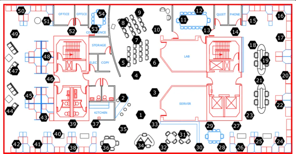
TinyOSplatform. The dataset contains 2.3 million pieces of sensory data collected by 54 nodes, including date, time, timestamp, node id, temperature, humidity, light, and voltage. Figure 1 shows the location distribution of 54 sensor nodes. Each sub-area has multiple sensor nodes to collect sensory data.
Node failure or data transmission errors sometimes occur in wireless sensor networks. In order to avoid the impact of abnormal data on the data prediction problem, this paper mainly deals with two forms of data outliers to improve data quality:
Global outlier: The data deviates from the range of the entire dataset.
Local outlier: The data is with the range of entire dataset, but abnormal compared with its
neighborhood.
Figure 2 shows an example to demonstrate these two kinds of data outliers. We consider the sine function with the normal data range as [−1, 1]. The value of node A is 1.2, which falls out of range [−1, 1]. In this case, we can say that the value of node A is a global outlier. On the other hand, the value of node B, 0, is regarded as a local outlier because it is in range of [−1, 1] and is abnormal with its neigh-boring data.
3.1 Global outliers processing
Global outlier has a great influence on data normalization and feature extraction, so it must beremovedbefore using the neural network to extract features of sensory data. In this paper, the quartile method is used to process the global outliers. First, find the lower quartile (Q1), median (Q2), and upper quartile (Q3) in the sensory data. Then, calculate the interquartile range (IQR), where IQR = Q3 −Q1. Fi-nally, calculate the lower fence (Q1 − 1.5IQR) and upper fence (Q3 + 1.5IQR), which are regarded as the lower and upper bound for the range of the entire dataset. In this way, the data which falls out of range [Q1 − 1.5IQR, Q3 + 1.5IQR] are considered as global outliers. In the Intel indoor dataset [30], there are four different types of data collected by the sensors, i.e., temperature, humidity, voltage, and light. We can obtain IQR and the upper and lower fences accord-ingly by calculating Q1, Q2, and Q3 for each given attribute. Figure3shows the boxplot for these four different at-tributes of node 8. The whiskers represent lower and
upper fences for each given attribute, and the red line inside the box is the median value. The collected data which falls out of the fences are marked with label + which means that they are outliers. As we can see from Fig.3, there are less outliers with the temperature attri-bute, while many outliers can be found with the voltage and humidity. Especially, most of the outliers of the humidity is close to the lower fence, while the outlier distribution of voltage is relatively scattered.
3.2 Local outliers processing
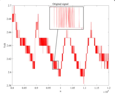
After the sensory dataset is processed by the quartile method, there are still a large number of local outliers, which generally appear different from their adjacent data although they are collected by the same node with the same attribute. The local outlier occurs sometimes due to the environmental noise which will influence the col-lected data in a random manner. Figure4shows the im-pact of noise on the data of node 8.
In order to reduce the noise influence on the data pre-diction problem, we adopt the wavelet threshold denoising to illuminate the noise in the original data. Wavelet threshold denoising can be divided into three sequential steps: wavelet decomposition, threshold acquisition, and wavelet denoising.
3.2.1 Wavelet decomposition
Given a 1-dimensional signal, in this paper, we use the multi-level wavelet decomposition in which the decom-position level is set to 4 (which is generally proposed in [31]), to obtain the wavelet decomposition coefficientC
and the coefficient length L which is used to calculate the threshold and while the multi-level decomposition is completed.
Fig. 2Classification of data outliers
Assuming that the input signal iss, the first step in the wavelet decomposition process of the signal s is shown in Fig.5. HiD and LoD represent the high-pass and low-pass decomposition filter separately, and↓2 presents the down-sampling process. In this way, the input signalsis converted to two outputs ascA1andcD1.
The decomposition process continues four times with the previous outputcAjas the input (Fig.6). Finally, we can obtain the coefficients [cA4,cD4, cD3,cD2,cD1] and the lengthLof each decomposition coefficient.
3.2.2 Threshold acquisition
In this paper, we use the unbiased risk estimation model to get the threshold of the one-dimensional wavelet transform. The threshold is calculated by the following steps:
a. Obtain the absolute value of each element in the signal; then, sort all the absolute values from small to large; finally, square the sorted data to get a new signalf(k), (k= 0, 1, 2, ...,N−1).
b. Calculate Risk (k) with Eq. (1) fork= 0, 1, 2, ... ,N
−1:
Riskð Þ ¼k
N−2kþX
k
i¼1
f ið Þ þðN−kÞf Nð −kÞ
N ð1Þ
c. Find the minimum one among these Risk(k),k= 0, 1, 2,... ,N-1, and let its square root be the final thresholdλ.
3.2.3 Wavelet denoising
The soft wavelet threshold denoising method uses differ-ent thresholds for denoising in each layer. The calculation process is:
wλ¼ sgnð Þw0;ðj jw−λÞ;j jw ≥λ
w
j j<λ
ð2Þ
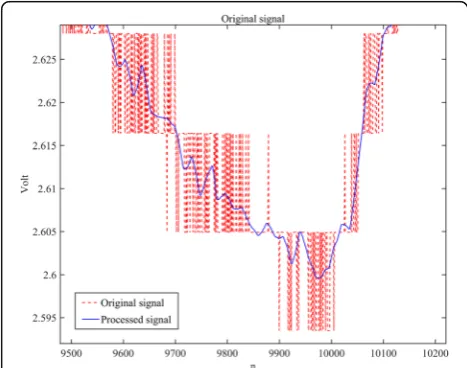
where w is the wavelet coefficient, λ is the pre-selected threshold, and sgn(·) is the sign function.wλis the wave-let coefficient filtered by the threshold function. Experi-ments have shown that the local outliers present are controlled after wavelet denoising [32–34]. Figure 7
shows the comparison between the original data and the data after wavelet denoising. Similar wavelet denoising process can be applied to different attributes of nodes in the network. In this way, we can finally get a wireless sensor network dataset with better data quality.
4 Correlation analysis
4.1 Data correlation in a single node
The Intel Indoor Dataset [23] contains a variety of sensory data collected by 54 nodes. In order to select appropriate sensory data to training the neural network and making the predictions reasonable, this paper takes the node 8 as an example to study the correlation of various sensory data and quantify the correlation. The sensory data used in this paper includes temperature, humidity, voltage, and light. Temperature is in degrees Celsius. Humidity is expressed in temperature corrected relative humidity, ran-ging from 0 to 100%. Light is in Lux, ranran-ging from 0 to 2000. Voltage is in Volt, ranging from 2 to 3. Considering the different range of several sensory data, in order to ex-tract the correlation features, this paper uses min-max normalization to linearly transform the sensory data to [0, Fig. 5Wavelet decomposition for signals
1]. The min-max normalization is calculated as shown in Eq. (3):
x0¼ x−xmin
xmax−xmin ð3Þ
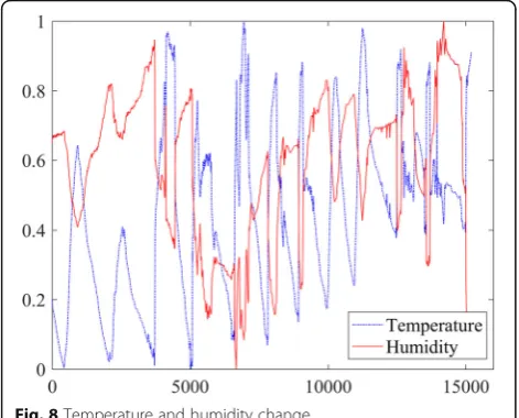
where x is the raw data, xmin is the minimum of the dataset,xmaxis the maximum of the dataset, andx'is the normalized data. After the normalization process, all sensory data is mapped to [0, 1]. Figure8shows the nor-malized temperature and humidity data.
According to the Fig. 8, there is a correlation between temperature and humidity. In order to improve the accuracy of the correlation analysis, this paper uses the Spearman correlation coefficient to quantify the correl-ation. The Spearman correlation coefficient is calculated as shown in Eq. (4):
ρ¼1− P
6d2i
n nð 2−1Þ ð4Þ
wherediis the difference between the two ranks of each observation.nis the number of observations.
Using the calculation Eq. (4) of the Spearman correl-ation coefficient, the correlcorrel-ation coefficient of temperature and humidity in node 8 is ρ =−0.4830. The correlation between various types of sensory data according to this method is shown in Table1.
Table1shows a strong correlation between temperature and humidity, temperature, and light, where temperature is negatively correlated with humidity and positively corre-lated with light. Humidity has a strong correlation with temperature and voltage, and humidity is negatively corre-lated with voltage.
4.2 Data correlation between multiple nodes
In order to get the spatial-temporal correlation between multi-node sensory data for neural network learning, this paper takes the node 8 as the center and selects the near-est node 7 and 9 to study the correlation of multi-node sensory data and quantizes it by Spearman’s correlation coefficient. The correlation of various types of sensory data among the three nodes is shown in Table2.
The same type of sensory data under multiple nodes has a strong correlation, and the temperature, humidity, and voltage are most obvious. From the position of node 8 and node 7 and node 9 in the wireless sensor network, the correlation of light data is mainly affected by the dis-tance between light source, the position of the shelter, and the orientation of the room. It is not suitable as a feature to train the spatial-temporal correlation-based prediction model.
Considering the sensory data correlation analysis of single-node and multi-node, this paper selects the temperature and humidity data of node 8 and the temperature data of nodes 7 and 9 as the input parame-ters of the spatial-temporal correlation-based prediction model, which is used to predict temperature data of node 8.
5 Method
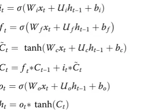
This section describes the features learning process of prediction model based on the two-directional LSTM neural network which is named as node multi-feature (MNMF) prediction model in this paper. As a special form of recurrent neural network (RNN), bidirec-tional LSTM neural network has a natural advantage in long-term memory [12–14]. Both LSTM and RNN have a chain structure consisting of a certain neural network module, which is called cell in LSTM. The cell consists of three gates: input gate, output gate, and forget gate. The structure of the cell used in this paper is as follows:
Fig. 8Temperature and humidity change
Table 1Correlation coefficient of sensory data
Correlation Temperature Humidity Voltage Light
Temperature 1.0000 −0.4830 0.0415 0.5617
Humidity -0.4830 1.0000 −0.5026 −0.2742
Voltage 0.0415 −0.5026 1.0000 0.2088
Light 0.5617 −0.2742 0.2088 1.0000
Table 2Correlation coefficient of multi-node
Correlation Temperature Humidity Voltage Light
No.8, no.7 0.9633 0.9726 0.9724 0.8674
No.8, no.9 0.9945 0.9909 0.9880 0.9180
it¼σðWixtþUiht−1þbiÞ ð5Þ
ft¼σ WfxtþUfht−1þbf
ð6Þ
~
Ct ¼ tanhðWcxtþUcht−1þbcÞ ð7Þ
Ct ¼ ftCt−1þitC~t ð8Þ
ot ¼σðWoxtþUoht−1þboÞ ð9Þ
ht ¼ottanhð ÞCt ð10Þ
Equation (5) is the input gate process, ht-1is the out-put of the previous cell, xtis the current cell input, σis the sigmoid function, andWi andUi are the input gate weights. Equation (6) is the function of forgot gate, which determines the information discarded in the cell, and Wfand Ufare the forgot gate weights. Equation (7) is a candidate memory unit that generates alternative updates. Equation (8) is the function of updating the cell state. The forgot gate decides what to be discarded in the old state information and adds the updated informa-tion to get the new state. Wc and Uc are the weights of the alternative new state, and * is the Hadamard prod-uct. Equations (9) and (10) are the output gate functions. Firstly, the sigmoid layer is used to determine the state of the cells to be output, then the updated cell state is processed by the tanh layer. Finally, the two parameters are multiplied to get the output, where Wo and Uo are weights of the output gate.
With the cell as the basic structure, this paper uses two-layer bidirectional LSTM neural network to construct the prediction model. Compared with the ordinary LSTM neural network, the bidirectional LSTM provides more local information to the network, which uses the forward and backward time series to get available information of timestamps in the past and future, so that it has better prediction result [15]. There is no direct connection be-tween the backward layer and the forward layer in Fig.9, ensuring that the expansion is acyclic. For the input layer
dataxt, the results of the forward and backward layers are combined at the output layer to get the output yt. The basic structure of the bidirectional LSTM is shown in Fig.9.
In wireless sensor networks, the sensory data collected by nodes has regional characteristics; in this way, the sensory data of different nodes have similar distribution patterns. Similarly, there is a correlation between different sensory data originated from the same node, which is rep-resented by a positive or negative correlation between various sensory data. In this paper, the spatial-temporal correlation of multi-node sensory data is used to construct a wireless sensor network data prediction model. As an example, the MNMF model structure is shown in Fig.10.
In Fig.10, Va and Vb are the temperature and humid-ity data of node 8. Vd and Ve are the temperature data of nodes 7 and 9. To extract the spatial correlation be-tween nodes, the timestamps of the node 8 needs to be exactly the same as nodes 9 and 7. LSTM1 is the first layer of bidirectional LSTM neural network that pro-cesses the input layer features and transmits them to the next layer. LSTM2 is the second layer of bidirectional LSTM neural network, which extracts abstract features from the previous layer. The FC is a fully connected layer, which performs the nonlinear transformation on the high-dimensional data in the previous layer. Merge is a fusion layer, which combines the abstract features of each node in the previous layer to predict temperature.
Since LSTM is used as the main structure of the pre-diction model, the shape of the input layer data needs to suit the parameter shape of the LSTM neural network, including the number of features input, the length of the time step, and the number of data. The stability and training speed of the prediction model need to be con-sidered when choosing the number of bidirectional LSTM neural network nodes. Too few neural network nodes are likely to cause insufficient training and under-fitting, and too many neural network nodes are likely to cause over-fitting and increase the duration of the model
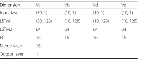
training. The length of the time step also has an effect on the prediction. The model dimensions adopted in this paper are shown in Table3.
In Table 3, the first dimension of the input layer and the LSTM1 layer is determined by the time steps of the specified feature, the time steps of Va are 50, and the time steps of Vb, Vd, Ve are 10. The length of the data sequence used by the LSTM model is determined by the time step. Using the appropriate time steps for different features can make the prediction model get a relatively good prediction. In this paper, the mean square error (MSE) is used as a loss function to estimate the devi-ation. The calculation process is as shown in Eq. (11):
Lð Þ ¼θ 1 m
Xm
i¼1
yi−^yi
ð Þ2 ð11Þ
whereθrepresents all parameters in the model,yi repre-sents the true value, and ŷi represents the predicted value. In this paper, the model uses the backpropagation algorithm to train and uses the Adam algorithm as the optimizer to calculate and update the network parame-ters. The adopted batch_size is set as 50, and the train-ing ends when the epochs of the traintrain-ing exceed 200. The model training process is described in Table4.
6 Results and discussion 6.1 Time step selection
In this paper, Tensorflow, Keras, and Matlab are used as the primary tools of the experiment, and GPU ac-celeration is used to train the model. By testing a var-iety of parameter configurations, it is found that the time step length has a great influence on the extrac-tion efficiency of data features in MNMF. If the se-quence is too short, the prediction model will get less information and can not make an accurate prediction. If the sequence is too long, the model will get too much information to extract useful feature from data. In this paper, 10, 20, 50, 100, 200, and other specific time steps are used as the basic unit of the combin-ation, the first 50% of the entire sensory dataset is used as the train set, and the last 50% is used as the test set to evaluate the prediction. Table 4 and 5 shows the relationship between the time step length
Table 4Training process of MNMF model
Table 3Feature shape of each layer in MNMF
Dimension Va Vb Vd Ve
Input layer (50, 1) (10, 1) (10, 1) (10, 1)
LSTM1 (50, 128) (10, 128) (10, 128) (10, 128)
LSTM2 64 64 64 64
FC 16 16 16 16
Merge layer 16
Output layer 1
Table 5Prediction deviation of multi-node multi-feature model
Timesteps Va Vb Vd Ve RMSE
100 200 10 10 10 0.201
100 10 10 10 0.160
100 20 10 10 0.172
100 20 20 20 0.248
100 10 20 20 0.424
50 10 10 10 0.139
10 10 10 10 0.290
50 100 10 10 10 0.443
50 10 10 10 0.101
20 10 10 10 0.156
of the multi-node multi-feature model (MNMF) and the prediction error, where Va and Vb are the temperature and humidity of node 8, and Vd and Ve are the temperatures of nodes 7 and 9.
The RMSE in Table 4 and 5 is the root-mean-square error, which is calculated as the square root of the Eq. (10). The root-mean-square error is used to measure the accuracy of the predicted value. This paper uses a variety of batch size training models and then compares them. Through the change of time step length and RMSE, it can be known that selecting a reasonable time step length is an effective way to improve the prediction effect. The pre-diction deviation of multi-node multi-feature model is de-scribed in Table5.
6.2 Feature selection
In the dataset used in this paper, there are many kinds of sensory data that can be used for prediction. Accord-ing to the correlation between data and experimental re-sults, the MNMF prediction model selects four features for prediction, in which Vb represents the temporal cor-relation between the data to be predicted and other sen-sory data of the same node, and Vd and Ve represent the spatial-temporal correlation between adjacent nodes. Va represents the temporal correlation between the data to be predicted and its historical data. In addition, this paper also constructs two prediction models based on single-node multi-features and multi-node single-fea-tures. The parameter configuration is similar to the MNMF model. The combination of the chosen sensory data and the length of the time step is shown in Tables 6and7.
Va shown in Table6is the temperature data sequence of node 8, Vb is the humidity data sequence, and Vc is the light data sequence. Since the sensory data of a single node is used, this model is called a single node multi-feature model (SNMF), where batch_size is set to 100. Table 6 shows the experimental results of the sin-gle-node model at each time step length, two extra-sen-sory data are used to extract useful correlation features, and the influence of the time step on the prediction is reasonable.
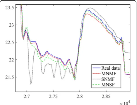
Va in Table 7 is the temperature data of node 8, Vd is the temperature data of node 7, and Ve is the temperature data of 9. Because using the same kind of sensory data in multiple nodes to train, it is called a multi-node single-feature model (MNSF) in this paper, and the batch size is set to 100 in training. Table 7 shows a prediction result that only consider-ing the correlation of the same kind sensory data in multiple nodes. Node 8 is in the same room with nodes 7 and 9 and they are close to each other so that the collected sensory data has a strong correl-ation. As shown in Table 2, the temperature data cor-relation coefficient between node 8 and node 7 is 0.9633, and the temperature data correlation between nodes 8 and 9 is 0.9945. The above results prove that constructing a prediction model using sensory data correlation in a wireless sensor network is an effective method. This paper combines the advantages of the above two models, constructing a node multi-feature model (MNMF). Figure 11 shows the partial sensory data prediction of the above three models.
6.3 Comparative experiment
To verify the performance of the model (MNMF), three neural network prediction models were used to compare the performance in the simulations.
Table 6Prediction deviation of single-node multi-feature model
Va Vb Vc RMSE
5 2 2 0.184
10 10 10 0.171
20 10 10 0.190
50 10 10 0.322
50 50 10 0.424
Table 7Prediction deviation of multi-node single-feature model
Va Vd Ve RMSE
5 2 2 0.174
10 10 10 0.159
20 10 10 0.140
50 10 10 0.213
50 50 10 0.305
1. Elman neural network. It is a typical local forward network (global feed forward local recurrent). The Elman network can be seen as a recurrent neural network with local memory units and local feedback connections.
2. NARX (nonlinear autoregressive exogenous model). The nonlinear autoregressive exogenous model mainly consists of four layers: input layer, hidden layer, bearing layer, and output layer, wherein the bearing layer uses a nonlinear autoregressive model with exogenous input.
3. GRNN (general regression neural network). A generalized regression neural network is an artificial neural network that uses a radial basis function as an activation function, which is an improvement of the radial basis network.
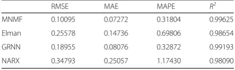
In order to improve the comprehensiveness of the evaluation, the root-mean-square error (RMSE), mean absolute error (MAE), mean absolute percentage error (MAPE), and R2 are used as evaluation indicators to evaluate the prediction model. RMSE is sensitive to out-liers that appear in prediction errors, while outout-liers in prediction errors have a relatively small impact on MAE, so RMSE and MAE are both used to evaluate the predic-tion. MAPE shows the ratio between the error and the actual value, which can be used to measure errors in dif-ferent orders of magnitude. R2is used to measure how well the regression prediction approximates to actual data, which is necessary for regression. Multi-type of evaluation indicators can estimate the quality of model predictions better and avoid incomplete evaluation, so the above four indicators are both used to evaluate the predictions. Equation (12) is the calculation process of MAE, Eq. (13) is the calculation of MAPE, and Eqs. (14), dicted value, y is the average value, andmis the number of samples. MAPE is the percentage of prediction bias and true value. Because the data range of each type of data is different, the calculated error is very different among vari-ous types of data. TheR2can be interpreted as the ratio of the predicted mean square error to the data variance. It represents the fitness of the predicted value and the actual value. The calculated evaluation indicators are shown in Table8.
The experiment shows that the MNMF model has a great advantage over Elman and NARX, and it has an advantage in RMSE andR2when compared with GRNN. Figure12shows the partial temperature data prediction curves of MNMF, GRNN, and Elman. Since the NARX neural network is obviously weaker than other models in various indicators, no further comparison is made here. It can be seen from Figure 12 that the MNMF model has lower prediction error and the prediction is more stable than the other two models.
7 Conclusion
The sensory data in the wireless sensor network is col-lected by multiple sensors of different nodes, which shows the relative variation of several environmental factors in different regions. In this paper, we quantify the correlation features between different sensory data and construct a
Table 8Predictive evaluation of multiple models
RMSE MAE MAPE R2
MNMF 0.10095 0.07272 0.31804 0.99625
Elman 0.25578 0.14736 0.69806 0.98654
GRNN 0.18955 0.08076 0.32872 0.99193
NARX 0.34793 0.25057 1.17430 0.98090
sensory data prediction multi-node multi-feature (MNMF) model, based on bidirectional LSTM. The model considers three factors including the temporal correlation between the sensory data and its historical data, the spatial correlation of the sensory data between different nodes, and the low data quality caused by the transmission error of the sensor network. Firstly, the quartile method and wavelet threshold denoising method are used to improve the data quality. Then, the bidirectional LSTM neural net-work is used to learn the prediction features respectively. Finally, the merge layer of the neural network is used to fuse multiple data features to predict the specific sensory data. In this paper, Intel indoor dataset is used for experi-mentation. The experiments show that the proposed MNMF model has high prediction accuracy and reason-able prediction bias.
Abbreviations
GRNN:General regression neural network; IOT: Internet of things; IQR: Interquartile range; LSTM: Long short-term memory; MAE: Mean absolute error; MAPE: Mean absolute percent error; MNMF: Multi-node multi-feature data prediction model; MNSF: Multi-node single-feature data prediction model; MSE: Mean square error; NARX: Nonlinear autoregressive exogenous; RMSE: Root-mean-square error; RNN: Recurrent neural network; SNMF: Single-node multi-feature data prediction model
Acknowledgements None.
Authors’contributions
HC proposed the framework of the data prediction strategy. Moreover, he also participated in the writing of this paper. ZX carried out the simulation and the initial idea of the MNMF. LW contributed to the data pre-processing. ZY discussed the framework and helped to improve the writing of this paper. RL provided the material and carried out the original data analysis. All au-thors read and approved the final manuscript.
Funding
This work is supported by the National Natural Science Foundation of China under Grand No. 61772136, 61370210, and the Science Foundation of Fujian Province under Grand No. 2019J01245.
Availability of data and materials None.
Competing interest
The authors declare that they have no competing interests.
Author details
1College of Mathematics and Computer Science, Fuzhou University, Fuzhou 350116, China.2Key Laboratory of Spatial Data Mining and Information Sharing, Ministry of Education, Fuzhou, China.3Fujian College Applied Engineering Centre of Internet of Things, Minjiang Teachers College, Fuzhou 350000, China.
Received: 22 March 2019 Accepted: 5 July 2019
References
1. P. Rawat, K.D. Singh, H. Chaouchi, J.M. Bonnin, Wireless sensor networks: a survey on recent developments and potential synergies. Journal of Supercomputing68(1), 1–48 (2014)
2. T. Railt, A. Bouabdallah, Y. Challal, Energy efficiency in wireless sensor networks: a top-down survey. Computer Networks67(8), 104–122 (2014)
3. H. Xiao, S. Lei, Y. Chen, H. Zhou,WX-MAC: An energy efficient MAC protocol for wireless sensor networks(2013 IEEE 10th International Conference on Mobile Ad-Hoc and Sensor Systems, Hangzhou, 2013), pp. 423–424 4. M.A. Razzaque, C. Bleakley, S. Dobson, Compression in wireless sensor
networks. Acm Transactions on Sensor Networks10(1), 1–44 (2013) 5. C.P. Chen, S.C. Mukhopadhyay, C.L. Chuang, M.Y. Liu, J.A. Jiang, Efficient
coverage and connectivity preservation With Load Balance for Wireless Sensor Networks. Sensors Journal IEEE15(1), 48–62 (2015)
6. Y. Song, J. Luo, C. Liu, W. He,Periodicity-and-Linear-Based Data Suppression Mechanism for WSN(2015 IEEE Trustcom/BigDataSE/ISPA, Helsinki, 2015), pp. 1267–1271
7. K.J. Yang, Y.R. Tsai,WSN18-2: Link Stability Prediction for mobile ad hoc networks in shadowed environments(IEEE Globecom 2006, San Francisco, 2003) 8. J. Kolodziej, F. Xhafa,Utilization of Markov model and non-parametric belief
propagation for activity-based indoor mobility prediction in wireless networks
(2011 International Conference on Complex, Intelligent, and Software Intensive Systems, Seoul, 2011), pp. 513–518
9. Q. Liu, D. Jin, J. Shen, Z. Fu, N. Linge,A WSN-Based Prediction Model of Microclimate in a Greenhouse Using an Extreme Learning Approach(2016 18th International Conference on Advanced Communication Technology (ICACT), Pyeongchang, 2016)
10. A. Sinha, D.K. Lobiyal, Prediction models for energy efficient data aggregation in wireless sensor network. Wireless Personal Communications
84(2), 1325–1343 (2015)
11. D. Spenza, C. Petrioli, A. Cammarano,Pro-Energy: A novel energy prediction model for solar and wind energy-harvesting wireless sensor networks(2012 IEEE 9th International Conference on Mobile Ad-Hoc and Sensor Systems (MASS 2012), Las Vegas, 2012), pp. 75–83
12. F. Karim, S. Majumdar, H. Darabi, S. Chen, LSTM fully convolutional networks for time series classification. IEEE Access6, 1662–1669 (2017)
13. A. Graves, N. Jaitly, A.R. Mohamed,Hybrid speech recognition with Deep Bidirectional LSTM(2013 IEEE Workshop on Automatic Speech Recognition and Understanding, Olomouc, 2013), pp. 273–278
14. K. Greff, R.K. Srivastava, J. Koutnik, B.R. Steunebrink, J. Schmidhuber, LSTM: a search space odyssey. IEEE Transactions on Neural Networks & Learning Systems28(10), 2222–2232 (2015)
15. Y. Yao, Z. Huang,Bi-directional LSTM recurrent neural network for Chinese word segmentation (International Conference on Neural Information Processing, 2016), pp. 345–353
16. H. Tian, S.C. Chen,MCA-NN: multiple correspondence analysis based neural network for disaster information detection(2017 IEEE Third International Conference on Multimedia Big Data (BigMM), Laguna Hills, 2017), pp. 268–275 17. F.X. Zhang, G.D. Li, W.X. Xu,Xinjiang Desertification disaster prediction
research based on cellular neural networks(2016 International Conference on Smart City and Systems Engineering (ICSCSE), Hunan, 2016), pp. 545–548 18. S. Traore, Y.F. Luo, G. Fipps, Deployment of artificial neural network for
short-term forecasting of evapotranspiration using public weather forecast restricted messages. Agricultural Water Management163(1), 363–379 (2016) 19. S.K. Biswas, N. Sinha, B. Purkayastha, L. Marbaniang, Weather prediction by
recurrent neural network dynamics. International Journal of Intelligent Engineering Informatics2(2/3), 166–180 (2014)
20. M. Makrehchi, S. Shah, W. Liao,Stock prediction using event-based sentiment analysis(2013 IEEE/WIC/ACM International Joint Conferences on Web Intelligence (WI) and Intelligent Agent Technologies (IAT), Atlanta, 2013), pp. 337–342
21. G. Dong, K. Fataliyev, L. Wang, One-step and multi-step ahead stock prediction using backpropagation neural networks (2013 9th International Conference on Information, Communications & Signal Processing, Tainan, 2013).
22. Z. Chen, X. Du, Study of stock prediction based on social network (2013 International Conference on Social Computing, Alexandria, 2013), pp. 913-916.
23. L. Wang, F.F. Chan, Y. Wang, Q. Chang,Predicting public housing prices using delayed neural networks(2016 IEEE Region 10 Conference (TENCON), Singapore, 2016), pp. 3589–3592
24. A.L. Teye, D.F. Ahelegbey, Detecting spatial and temporal house price diffusion in the Netherlands: a Bayesian network approach. Regional Science and Urban Economics65, 56–64 (2017)
26. Y. Lv, Y. Duan, W. Kang, Z. Li, F.Y. Wang, Traffic flow prediction with big data: a deep learning approach. IEEE Transactions on Intelligent Transportation Systems16(2), 865–873 (2015)
27. W. Huang, G. Song, H. Hong, K. Xie, Deep architecture for traffic flow prediction: deep belief networks with multitask learning. IEEE Transactions on Intelligent Transportation Systems15(5), 2191–2201 (2014)
28. R. Fu, Z. Zhang, L. Li,Using LSTM and GRU neural network methods for traffic flow prediction(2016 31st Youth Academic Annual Conference of Chinese Association of Automation (YAC), Wuhan, 2016), pp. 324–328
29. X. Dai, R. Fu, Y. Lin, L. Li,DeepTrend: A deep hierarchical neural network for traffic flow prediction(2017 20th International Conference on Intelligent Transportation Systems, Yakahama, 2017)
30. Intel. Intel Lab Data.http://db.csail.mit.edu/labdata/labdata.html. Accessed 19 Apr 2019.
31. K. Kannan, S.A. Perumal,Optimal decomposition level of discrete wavelet transform for pixel based fusion of multi-focused images(International Conference on Computational Intelligence and Multimedia Applications (ICCIMA 2007), Sivakasi, 2007), pp. 314–318
32. R. F. Navea, E. Dadios, Classification of wavelet-denoised musical tone stimulated EEG signals using artificial neural networks (2016 IEEE Region 10 Conference (TENCON), Singapore, 2016), pp. 1503-1508.
33. J. Zhao, J. Huang, N. Xiong, An effective exponential-based trust and reputation evaluation system in wireless sensor networks. IEEE Access7, 33859–33869 (2019)
34. W. Guo, Y. Shi, S. Wang, N. Xiong, An unsupervised embedding learning feature representation scheme for network big data analysis. IEEE Transactions on Network Science and Engineering, 1–14 (2018)
Publisher’s Note