3D Visualization of Radar Backscattering
Diagrams Based on OpenGL
Yulia V. Zhulina
Interstate Joint Stock Corporation “Vympel,” P.O. Box 83, Moscow 1010001, Russia Email:yulia [email protected]
Received 20 May 2003; Revised 13 October 2003; Recommended for Publication by Xiang-Gen Xia
A digital method of calculating the radar backscattering diagrams is presented. The method uses a digital model of an arbitrary scattering object in the 3D graphics package “OpenGL” and calculates the backscattered signal in the physical optics approxima-tion. The backscattering diagram is constructed by means of rotating the object model around the radar-target line.
Keywords and phrases:radar scattering, backscattering diagrams, physical optics.
1. INTRODUCTION
The task, which represents a constant interest in radioloca-tion, is constructing a scattering diagram of an object illu-minated by a radar. This task has been resolved more than once by the accurate mathematical methods of electrody-namics [1,2,3], by experimental modeling of the radar sys-tems [4,5], by digital modeling of irradiated objects as com-bination of elements with known backscattering diagrams (such as pieces of the flat plates) [6,7,8,9,10]. The various methods for electromagnetic field modeling are comprehen-sively summarized in [11]. A review of generalized moment methods in the differential equations of electromagnetics is given in [12].
At present, the first method widely uses the numerical solution of the problem. Digital electromagnetics simulation allows accurate modeling of physical systems in combination with an accurate numerical solution of either differential or integral formulations of Maxwell’s equations. This compu-tational electromagnetics can be applied to many practical engineering problems, for example, antenna design, calcu-lation, backscattering diagrams, targets recognition, and so forth. However, the accurate analysis and synthesis of com-plex electromagnetic systems have remained beyond the lim-its of computer capabilities up to now.
The most reliable approach has always been a method of natural modeling. It means that the model of object, con-structed of real metallic or other materials, is irradiated by a real radar transmitter, and a real radar receiver gets the scattered signals. In this case, the very important thing is to keep the necessary proportions between the irradiated wave-length, the sizes of the object model, and the distance
be-tween the radar and the object. These conditions are not al-ways feasible. Besides, the natural and analog modeling are rather expensive and available for big organizations such as the White Sands Missile Range (WSMR), which possesses a highly specialized range instrumentation, technical laborato-ries, and facilities to support the continuing testing of NASA foreign and commercial systems. The modeling capabilities of the complex include tools for performing electromagnetic analysis, simulating electromagnetic wave propagation, and calculating antenna patterns. By the way, NASA publishes data of experimental measurements of radar cross sections for different shapes of radar targets [13].
the element approach to curved patches [15] although most of the works employ flat piecewise representation.
In this article, the method which represents the digital modeling of an object with the use of 3D graphics pack-age “OpenGL” is proposed. This method simulates a scalar electromagnetic radiation of the object, but this task may be modeled also in the case of the polarized irradiation.
2. THE FORMULA DESCRIPTION OF THE SCATTERED SIGNAL
In the approximation of physical optics, the complex ampli-tude of a signal, reflected by a target and received by the radar position, disposed in the pointR0, can be described by the
Kirchhoffintegral [16,17,18]. An approximate derivation of the Kirchhoffintegral theorem is given in the appendix. If the locations of the transmitter and the receiver coincide (R0=R1), the complex amplitude of the received signal can
be described by the formula (up to a constant complex mul-tiplier) the point of the object,
Fr=0 (2a)
is the equation of the surface of object,
η(x)=
is the distance from the pointrto the point of the radar po-sitionR0,λis the length of the wave of the radar irradiation,
andn(r) is the vector of the exterior normal to the surface of the object in the point r. For the visible part of object
−n(r)·((r−R0)/|r−R0|)>0 always.
If we could model the integral (1) in the various aspects of an object to the radar, we would get the scattering diagram of the object illuminated by the radar with wavelengthλ.
3. DESCRIPTION OF THE MODEL
Practically, any 3D object can be modeled in the package OpenGL. This package allows to build spheres, cylinders, cones, prisms, polygons, and lines. Most complex objects can be constructed of all these elements. The every point of the surface of the constructed object has a 3D description in the
Computer
Figure1: The whole scene of the model.
package: a two-dimensional (2D) position of the point on the computer screen (X,Y) and the distance of the point to the screen (Zcoordinate). The object can be rotated relatively in any point in the space in an arbitrary way. It can be irradiated by the source of illumination disposed in an arbitrary space point. All these program properties permit to exactly simu-late the radar system practically. And this package is suitable enough for calculating the backscattering diagram of the ob-jects with various shapes. The calculation procedure is as fol-lows.
(1) The object is placed on the screen plane and the radar irradiates the object in the direction perpendicular to the screen.
The irradiating scene and the model elements are shown inFigure 1. The position of the center mass of the object will be designed asr0, and this pointr0lies in the screen (in the
center of the window which is to be processed). For each real point of the objectr, we will introduce the screen coordinates
r=r−r0. (2c)
(2) Every point of the objectr, visible in the screen, has coordinates (X,Y) in the screen and coordinateZ(its distance from the screen).
(3) Every point of the objectr, disposed on its surface and visible in the screen, gives a complex scattered ampli-tudeA(r) in the point of radarR0:
In the process of modeling, we will suppose the vector
r−R0as follows:
r0−R0=r0−R0e, (4)
wheree=(0, 0, 1) is the normalized vector of the direction of the radar irradiation, directed perpendicularly to the screen.
The multiplier−n(r)·((r0−R0)/|r0−R0|) is created
automatically in the process of the 3D object modeling, as the package OpenGL simulates 3D objects and takes into account the direction of light source irradiation. So, we can get the value of intensityE(X,Y) of the screen pixel with the screen coordinates (X,Y):
For getting the visible part of the surface, the package calcu-lates only valuesE(X,Y)>0. If the object is disposed in a far zone, the condition is true:
r−r0=rr
0−R0, (6)
and we can write the distance of each point to the radar as follows:
r−R0=r+r0−R0≈Z0+Z. (7)
HereZ0 = |r0−R0|is the distance from the screen to the
radar andZis the distance of the point to the screen. So (3) can be rewritten as follows:
A(X,Y,Z)=A0
(4) We must summarize all the amplitudes (8) over the whole visible and illuminated part of the object sur-face to get the whole signal received by the radar from the rangeZ:
Ziis the distance from the screen of the pixel with the screen coordinatesXi,Yi andI is the whole summa-rized number of pixels in the visible part of the object surface.
(5) To get the signal S0 received by the radar, we have
to summarize the signals (9) over all the band of the range values and calculate the total amplitude:
S0=
whereMis the whole number of the discrete ranges in the band of ranges.
(6) Notice that the signalS0is the function of the angles of
the object rotation relative to the radar, that is,
S0=S˜0(α,β,γ), (12)
whereα,β, andγare the angles of rotation around axes Y,X, andZ, correspondingly. If the object is an axis-symmetrical body, then expression (12) is the function of the single angleαbetween the axis of symmetry and directione(formula (4)) to the radar:
S0=S˜0(α). (13)
In this case, the construction of the scattering diagram leads to the calculation of all the meanings (13) over the whole range of valuesα. And this sequence is the scattering diagram.
4. THE RESULTS OF THE DIGITAL MODELING
The process of calculations consists of the following opera-tions:
(1) rotating the object around the vertical axisYat the an-gleα. In all the figures, the axisY is directed from the bottom to top;
(2) calculating the complex signal (8) from each pixel of the screen belonging to the visible part of the object; (3) summarizing these signals from the pixels lying at the
same distanceZ from the screen by formula (9). As a result, we get a coherent complex wideband signal from the object;
(4) accumulating signals of all ranges and calculating the amplitude of the signal by formula (11);
(5) recording the diagram for valueα;
(6) calculating the new angleαfor the new object aspect; (7) transfering to the point of calculations (1).
The results of modeling are shown in Figures2,3,4,5,6, and 7for the sphere, cylinder, cone, and object representing the combination of the cone and cylinder.
In all the figures, the relative position of the object to the screen (just the same as to the radar) is shown at the moment of getting the current point of the diagram. The graphic of the diagram is being drawn moving with a discrete of angle αequal to delα=0.5◦(Figures2,3,4,5,6, and7).
The initial angleα=45◦in all the figures and the mean-ings ofαare decreasing (rotating overy-axis in the clockwise direction).
Figure2: The whole scattering diagram of the sphere (45◦÷45◦− 360◦).
Fi=270
Fi=180
Fi=0
Fi=90
Figure3: The whole scattering diagram of the cylinder (45◦÷45◦− 360◦).
Fi=197
Fi=270
Fi=343
Fi=90
Figure4: The whole scattering diagram of the cone (45◦÷45◦− 360◦).
Fi=180
Fi=197
Fi=270
Fi=343
Fi=0
Fi=90
Figure5: The whole scattering diagram of the cone-cylinder com-position (45◦÷45◦−360◦).
Figure 6: Signal in the direction of the normal to the surface of cylinder in the cone-cylinder composition.
5,6, and7. Some of the objects are increased in sizes for the better visualization of the figures.
In Figures 3, 4, and 5, the angle values Fi are shown, which are equal to the corresponding value of angleαat the moment.
All the calculations have been performed in the windows with the dimension of 360×360 pixels in Figures2,3, and 4, and in Figures5,6, and7in the window with the size of 400×400 pixels. The width of the single pixel was taken equal toλ/15.0 in all the calculations.
Figure 2 shows the diagram from the sphere, which is constructed by 32 vertical slices. The radius of the sphere is equal to 50 pixels.Figure 2shows the whole diagram when angleαbecomes equal toα =45◦−360◦ and the sphere is turned at the angle of−360◦.
FromFigure 2, it is seen that the signal repeats itself 32 times round they-axis. It matches the reflection from the 32 identical slices. If the number of slices streams to infinity, the sphere will be entirely smooth and its signal will be the same in all the directions.
Figure 3shows the diagram of a cylinder. The cylinder is 200 pixels long and it has radius of 30 pixels. As the cylinder is an axis-symmetrical body, all the diagram is symmetrical rel-ative to the main maximum. This maximum is received from the lateral surface of the cylinder as the lateral surface has the maximal radar cross section (in this example). This max-imum is the narrowest among the others because the height of the cylinder is approximately 3 times more than the diam-eter of the bottom.
Two maximums of the second magnitude are produced by the bottom of the cylinder.
InFigure 3, the cylinder is turned to the angle of−360◦ from its start angle positionα=45◦.
Figure 4shows the diagram of a cone. The cone is 100 pixels long and has a bottom radius of 30 pixels. As the cone is an axis-symmetrical body, all the diagram is symmetrical relative to the main maximum. This maximum is received from the bottom of the cone, as the bottom has the maximal radar cross section (in this example). This maximum is the widest among the others because the diameter of the bottom is∼1.7 times less than the height of the cone.
Two maximums of the second magnitude are produced by the flank of the cone when the direction to the radar re-ceiver has the perpendicular angle to the flank surface of the cone. At this moment,αbecomes equal toα=β, where 2βis an angle at the top of the cone andβ=arctg(0.3)≈17◦, and the cone is turned at the angle ofβ−45◦= −28◦.
The two more small maximums of the diagram are ob-tained when the visible part of the cone has the largest sur-face, but the normal is not directed to the radar receiver.
At last, the smallest maximum is provided by the nose of the cone from the direction opposite to the direction of the main maximum.
InFigure 4, the cone is turned to the angle of−360◦from its start angle positionα=45◦. Figures5,6, and7show the diagram from a cone plus a cylinder composition. The cylin-der is 200 pixels long and has a radius of 30 pixels. The cone is 100 pixels long and has a bottom radius of 30 pixels. The
0 20 40 60 80 100 120 140 160 180 200 −50
−40 −30 −20 −10 −0 10 20
Figure8: The scattering diagram of the cone-cylinder composition obtained by the method of flat plates.
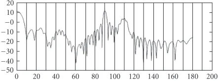
0 20 40 60 80 100 120 140 160
4.00 5.01 6.03 7.04 8.06
Figure9: The scattering diagram of the cone-cylinder composition obtained by using OpenGL package.
composition is also the axis-symmetrical body and all the di-agram (Figure 4) is symmetrical relative to the maximum re-ceived from the bottom of the cylinder.
The main maximum is given by the lateral surface of the composition at the moment when the direction to the radar receiver has the perpendicular angle to the lateral surface of the cylinder. All the construction has the maximal radar cross section in this aspect. This maximum is the narrowest among the others as the length of the construction is more than the diameter of the cylinder bottom.
Two maximums of the second magnitude are produced by the flank of the cone when the direction to the radar re-ceiver has the perpendicular angle to the flank surface of the cone. The central maximum is provided by the bottom of the cylinder.
Figure 5shows the whole diagram when angleαbecomes equal to 45◦−360◦and the construction is turned at the angle of−360◦.
Figures 6and7 are given as an illustration of process-ing the diagrams. The drawprocess-ings of the diagrams built until the moment and the aspect of the construction at the mo-ment are shown.Figure 6shows the maximum of the dia-gram from the lateral side of the cylinder when the direction to the radar receiver has the perpendicular angle to the lateral surface of the cylinder. At this moment,αbecomes equal to 0◦and the whole construction is turned at the angle of−45◦. Figure 7shows the maximum of the diagram from the bottom of the cylinder.
[19]. Correspondingly, in Figure 9, the diagram of cone-cylinder (Figure 5) is unrolled in the angle space. The posi-tions of maximums from the flank surface of the cone are different because the cone in Figure 8has the angle at its top equal to 40◦, and inFigure 9, it is equal to 34◦. A ratio λ/Dim, where Dim is a size of the whole object, is higher in Figure 8. That is why all the lobes inFigure 8are wider than inFigure 9. The diagram inFigure 8is given in dB/m2;
in other words, it is normalized to the cross section, and in Figure 9, it is given simply in logarithmic scale. But the whole pattern of the diagrams is the same.
There is a need to say that accurate building of diagrams with thorough drawing all the side lobes is achievable only when the ratio of each pixel width to the wave lambda λ is small enough. In the calculations of the paper, this ra-tio was taken equal to 1/15. So the accurate calculara-tion of the large objects diagrams will demand the displays of large sizes.
5. DISCUSSION
The digital modeling of the physical optics integral (1) by the 3D graphics methods gives results (Figures2,3,4,5,6, and7) rather close to those obtained by the methods of flat places [19]. The described approach seems to be much less labor-intensive because it uses the ready-made 3D model of the object, and the algorithm only substitutes the coordinates and intensity of the screen pixels into the sum (9).
Using the flat places, approximation includes both the construction of an object and the calculation of (1). The whole volume of the works using this method can be es-timated from [8,9]. Some steps have to be made: the first step is the definition of the whole set of the object flat plates; the next one is the analysis of elementary flat plates visible from the radar, and the calculation of the radar cross sec-tion of each scattering center of the object as funcsec-tion of flat plate orientation and position. After this, the complex echo signal received from each center and the total power of the echo signal for each radar resolution cell are calcu-lated.
As it has been previously mentioned, the nature model-ing may appear to be expensive or not available in the condi-tions of the theoretical laboratories.
As for the method of building backscattering diagrams by means of numerical solutions of Maxwell’s equations, it should be mentioned that the equations are usually digi-tized with the help of a set of known expansion functions. This leads to a linear system of equations withNunknowns, whereNis the number of expansion functions. In this case, the computer requirements are at least proportional to N2
in terms of both computer time and memory. SinceNmay be very large, these requirements are beyond the capabili-ties of today’s computers (e.g., 76 GB RAM ifN =100.000) [20,21].
To resolve the problem, researchers have developed the fast multipole method (FMM) and the multilevel fast mul-tipole algorithm (MLFMA) [22,23,24]. It has been demon-strated that, using this MLFMA procedure, the calculations
can be performed with orderNlogNcomplexity. Addition-ally, improved MLFMA approach is developed in [25]. This approach is more efficient computationally, especially as the number ofNincreases.
In the presented method of modeling, the main compu-tational requirements are imposed on the speed of reading pixels from the screen, in other words, on the speed of per-forming the OpenGL functions. The whole diagram of 720 points with reading all the pixels in the window of 400×400 pixels was calculated in 4.5 minutes at the computer with 256 MB RAM and 1300 MHz clock rate.
By the way, the method calculates the wideband signal in the process of building diagram (formula (9)), which can be used in a lot of radar simulation software.
So the presented results allow to draw a conclusion that the digital modeling of object with the use of 3D graphics package OpenGL gives opportunity of simulating electro-magnetic radiation of the object. This method can reduce the workload of radar data simulation by using 3D graphics package constructed by many compilers. This method can be used by researchers who have no radar data simulation soft-ware.
The algorithm, proposed in this article, requires the pre-sentation of the object with the dimensions of pixels much less than the length of waveλfor the proper working. It is only the serious restriction on the method because a large object consists of large number of pixels and it will enlarge the time of calculations and will require a big display.
APPENDIX
The Fresnel-Kirchhoffapproximation to diffraction is well known [16,17, 18]. It is Fresnel diffraction principle that states that every unobstructed point of a wavefront, at a given instant time, serves as a source of spherical secondary waves (with the same frequency as that of the primary wave). The amplitude of the field at any point beyond is the superpo-sition of all these waves (considering their amplitudes and phases). This rather hypothetical principle has been later on developed in a more rigorous way by Kirchhoff, who proved that it can be derived from the scalar diffraction theory.
Consider a radar transmitter and a receiving position dis-posed in the pointsR0andR1, respectively.
The electromagnetic field at the receiver is a solution of the wave equation
∇2
P= 1
c2
∂2P
∂t2. (A.1)
We can express the solution in the formP(t,R)=P˜(R)ejkct (wherecis the light speed, k = 2π/λis the wave number, λ is the wavelength,ω = kc). Substituting this in the wave equation, we obtain the Helmoltz equation:
∇2P˜+k2P˜=0. (A.2)
terms of the field and its gradient assigned on an arbitrary scattering surfaceSenclosingR1:
˜
which is known as the Kirchhoffintegral theorem.
In (A.3),r designates the coordinates of the surface S point,dSis the differential of the surface, and∇n(r)f(r)
des-ignates the gradient of f(r) along the normaln(r) to the surfaceSin the pointr. The boundary conditions ˜P(r)|Sand
∇n(r)P˜(r)|Scan be chosen as the values of the primary spher-ical wave irradiated by the transmitter and its gradient pro-jections to the vectorn(r), respectively.
The primary radiated spherical wave in the surface point
the unit distance from the transmitter.
By direct calculations of (A.3), we can obtain the expres-sion for the field in the point of observationR1:
˜
the transmitter and the receiver, respectively,
[1] R. G. Kouyoumjian and P. H. Pathak, “A uniform geometrical theory of diffraction for an edge in a perfectly conducting sur-face,”Proceedings of the IEEE, vol. 62, no. 11, pp. 1448–1461, 1974.
[2] D. E. Kerr, Ed., Propagation of Short Radio Waves, Peter Pere-grinus, London, UK, 1987.
[3] D. A. McNamara, C. W. I. Pistorius, and J. A. G. Malherbe, Introduction to the Uniform Geometrical Theory of Diffraction, Artech House, Boston, Mass, USA, 1990.
[4] W.-M. Boerner, M. B. El-Arini, C.-Y. Chan, and P. M. Mas-toris, “Polarization dependence in electromagnetic inverse problems,”IEEE Trans. Antennas and Propagation, vol. 29, no. 2, pp. 262–271, 1981.
[5] N. N. Bojarski, “A survey of physical optics inverse scattering identity,” IEEE Trans. Antennas and Propagation, vol. 30, no. 5, pp. 980–989, 1982.
[6] A. I. Ladygin and A. A. Lychin, “Physical optics resolving an inverse diffraction task for the rough objects,”Electromagnetic Waves & Electronic Systems, vol. 5, no. 2, pp. 238–251, 2000, (Russian).
[7] Z. Sipus, P.-S. Kildal, R. Leijon, and M. Johansson, “An al-gorithm for calculating Green’s functions of planar, circular cylindrical and spherical multilayer substrates,”Applied Com-putational Electromagnetics Society Journal, vol. 13, no. 3, pp. 243–254, 1998.
[8] G. Galati, M. Ferri, and F. Marti, “(1994) advanced radar techniques for the air transport system: the surface movement miniradar concept,” in1994 IEEE National Telesystems Con-ference, (NTC ’94), San Diego, Calif, USA, May 1994. [9] G. Galati, M. Ferri, P. Mariano, and F. Marti, “(1994)
advanced integrated architecture for ground movements surveillance,” in1995 IEEE International Radar Conference, Alexandria, Va, USA, May 1995.
[10] M. D. Deshpande, C. R. Cockrell, F. B. Beck, E. Vedeler, and M. B. Koch, “Analysis of electromagnetic scattering from ir-regularly shaped, thin, metallic flat plates,” Nasa TP-3361, NASA Langley Research Center, Hampton, Va, USA, Septem-ber 1993.
[11] E. K. Miller, “A selective survey of computational electromag-netics,”IEEE Trans. Antennas and Propagation, vol. 36, no. 9, pp. 1281–1305, 1988.
[12] J. J. H. Wang,Generalized Moment Methods in Electromagnet-ics, John Wiley & Sons, NY, USA, 1991.
[13] A. C. Woo, H. T. G. Wang, M. J. Schuh, and M. L. Sanders, “em programmer’s notebook-benchmark radar tar-gets for the validation of computational electromagnetics pro-grams,”IEEE Antennas and Propagation Magazine, vol. 35, no. 1, pp. 84–89, 1993.
[14] S. M. Rao and D. R. Wilton, “Transient scattering by con-ducting surfaces of arbitrary shape,” IEEE Trans. Antennas and Propagation, vol. 39, no. 1, pp. 56–61, 1991.
[16] M. Born and E. Wolf, Principles of Optics, Pergamon Press, NY, USA, 6th edition, 1980.
[17] E. Hecht, Optics, Addison Wesley, Reading, Mass, USA, 2nd edition, 1987.
[18] J. B. Keller, “Geometrical theory of diffraction,”Journal of the Optical Society of America, vol. 52, no. 2, pp. 116–130, 1962. [19] A. I. Ladygin, Theoretical Bases of the Space Objects
Recogni-tion with the Radar ObservaRecogni-tion, Moscow AviaRecogni-tion Institute, Moscow, 1997, (Russian).
[20] E. Jørgensen, S. Maci, and A. Toccafondi, “Fringe integral equation method for a truncated grounded dielectric slab,” IEEE Trans. Antennas and Propagation, vol. 49, no. 8, pp. 1210–1217, 2001.
[21] E. Jørgensen, P. Meincke, and O. Breinbjerg, “An efficient fringe integral equation method for optimizing the antenna location on complex bodies,” inIEEE Antennas and Propaga-tion Society Symposium, pp. 584–587, Boston, Mass, USA, July 2001.
[22] J. M. Song, C. C. Lu, and W. C. Chew, “Multilevel fast mul-tipole algorithm for electromagnetic scattering by large com-plex objects,” IEEE Trans. Antennas and Propagation, vol. 45, no. 10, pp. 1488–1493, 1997.
[23] X. Q. Sheng, J. M. Jin, J. Song, W. C. Chew, and C. C. Lu, “Solution of combined field integral equation using multilevel fast multipole algorithm for scattering by homogeneous bod-ies,” IEEE Trans. Antennas and Propagation, vol. 46, no. 11, pp. 1718–1726, 1998.
[24] N. Geng, A. Sullivan, and L. Carin, “Fast multipole method for scattering from an arbitrary PEC target above or buried in a lossy half space,”IEEE Trans. Antennas and Propagation, vol. 49, pp. 740–748, May 2001.
[25] Z. Liu, R. J. Adams, and L. Carin, “New MLFMA formulation for closed PEC targets in the vicinity of a half space,” submit-ted to IEEE Trans. Antennas and Propagation.
Yulia V. Zhulinawas born in Igarka, Rus-sia. She graduated from the Moscow Physi-cal and Engineering Institute, Moscow, Rus-sia, in 1963. She received her Ph.D. degree in radar engineering from the Moscow Physi-cal and Engineering Institute, Moscow, Rus-sia, in 1968. In 1963, she joined the Radar Engineering Department at Vympel com-pany, where she is currently a Senior Sci-entist Researcher. She is the coauthor of the