Candidate main field models for producing the 9th generation IGRF

Candidate main-field models for producing the 9th generation IGRF

Mioara Mandea∗

Institut de Physique du Globe de Paris, 4 place Jussieu, 75252 Paris Cedex 05, France

(Received January 11, 2005; Revised May 3, 2005; Accepted May 3, 2005)

This paper presents the various candidate models used in deriving the 9th generation IGRF. Based on notes submitted to the IAGA working group V-MOD with the Gauss coefficients, a brief description of the data used and the method of modelling for each of the candidate models is given. The six candidate models for epoch 1995.0 and the five for epoch 2000.0 are presented. Improvements gained by the new models are also discussed.

Key words:IGRF, DGRF, modeling, core field, secular variation.

1.

Introduction

The largely non-specialist community of users favours an established, regular routine for updates of the IGRF models and for designation of the DGRF models. One of the central issues is to collect candidate models for the new IGRF or DGRF, evaluate the candidate models, and adopt the final IGRF or/and DGRF models. Generally, this occurs every 5 years, and is one of the main tasks of the IAGA work-ing group, for time bework-ing named V-MOD, formerly called V-8 Analysis of the Global and Regional Field and its Sec-ular Variation. The large community using these models have already stated clearly that it is necessary to preserve simplicity and ease of identification of the standard. There-fore, the working group V-MOD maintains the traditional 5-year recipe, except for the 9th generation IGRF which was revised after only 3 years (for more details see the web page1_{), with a spherical harmonic expansion for the} main-field model up to degree/orderNi =10 (for models prior to 2000), orNi =13 (for models starting in 2000), and with an expansion for the predicted secular variationNSV =8.

In this paper a summary, in a standard form, of the vari-ous candidate models for the 9th generation IGRF is given. Based on notes submitted to V-MOD with the Gauss co-efficients, a brief description of the data used and method of modelling for each of the candidate models is given (for the most complete description of candidate models see the web page2_{. The aim of this work is to preserve information} about the candidate models considered in producing the 9th generation IGRF, as only a few of them are presented in this issue. Each candidate model is identified by the name attributed during the evaluation processes. Table 1 summa-rizes the candidate models for the 9th generation IGRF.

∗_{Now at GeoForschungsZentrum Potsdam.}

Copyright cThe Society of Geomagnetism and Earth, Planetary and Space Sci-ences (SGEPSS); The Seismological Society of Japan; The Volcanological Society of Japan; The Geodetic Society of Japan; The Japanese Society for Planetary Sci-ences; TERRAPUB.

2.

Candidate Models for the Epoch 1995.0

This model was proposed byA. Thomson and S. Macmil-lan.

Data The dataset used covers the 1991–1999 time span and it contains near-Earth and total field satellite data pro-vided by POGS satellite.

Annual mean X,Y,Zvalues for 1991–1998 from obser-vatories were selected. Crustal biases were computed where possible, by comparison of the 1999 annual means with an Ørsted-only based model. For 150 observatories these crustal biases were deducted and removed from the annual means; for 55 no bias corrections have been applied.

Repeat stations occupied between 1991.0–1999.0 were also used. After removing outliers and observations with large crustal fields, based on comparison with 8th gener-ation IGRF and eliminating stgener-ations with|Z,F| residuals

≥ 500 nT and|X,Y| residuals≥ 500√2 nT, 1320 repeat stations were kept. Some 90 one-off surveys were added, after processing them in the same way.

From 1993.05 to 1994.23 one-minute mean values of Project MAGNET aeromagnetic vector observations were considered. After selection over periods when the geomag-netic planetary three-hour-range index Kp is Kp<2+and after applying the same rejecting criteria as for the repeat stations, 22640 data were used.

Marine total intensity data covered 1991.0–1999.0 pe-riod. The final 4473 marine data were obtained after select-ing every second point along survey tracks; 110 km along-track means were computed from a minimum 25 data with Kp≤2+and|F|residuals≤500 nT when comparing with the 8th generation IGRF.

POGS satellite scalar data, between 1991.03–1993.58, were selected according to the following criteria: Kp≤1+,

−15≤Dst ≤ +5 (whereDstis a geomagnetic index which monitors the world wide magnetic storm level), 22:00 ≤ local time≤05:00, solar zenith angle filtered (data rejected where ionosphere below satellite is sunlit), and an outlier rejection for|F|residuals≥100 nT when comparing with

1_{http://www.iugg.org/IAGA/iaga pages/science/division 5.htm.} 2_{http://www.ipgp.jussieu.fr/ mioara/dgrf/dgrf page.html.}

Table 1. Candidate models for the 9th generation IGRF.

Model-Abbreviation Authors (countries)

DGRF1995-BGS Thomson and Macmillan (UK)

DGRF1995-CM Olsen, Lowes, Sabaka (Denmark, UK, USA)

DGRF1995-GFZ Maus, L¨uhr, Rother, Mai, Mandea (Germany, France)

DGRF1995-GFZ2 Wardinski and Holme (Germany, UK)

DGRF1995-IPGP Chambodut, Langlais, Mandea (France, USA)

DGRF1995-IZM Bondar and Golovkov (Russia)

DGRF2000-BGS Lesur, Thomson, Macmillan (UK)

DGRF2000-CM Olsen, Lowes, Sabaka (Denmark, UK, USA)

DGRF2000-OSVM Olsen, Lowes, Sabaka (Denmark, UK, USA)

DGRF2000-GFZ Maus, L¨uhr, Rother, Mai (Germany)

DGRF2000-IPGP Chambodut, Langlais, Mandea (France, USA)

the 8th generation IGRF. Both the near-surface and satellite datasets were further decimated by selecting separately a maximum 7 data locations per equal-area tessera of which there were 1654 covering the Earth’s surface. The selection used the magnetically quietest data and for the near-surface data used those from observatories, repeat stations, one-off surveys, Project MAGNET and marine surveys in that order.

Modelling method Data were weighted in the model solution. The relative weights for both satellite and sur-face data, in terms of data quality and crustal field signa-ture, were determined by iteratively re-weighting the input data according to fits to interim models, derived at each step of a six stage iteration process. Equal-area weighting was also applied to all data. All data were reduced to the epoch 1995.0 prior to main-field model derivation, using annual secular-variation models prepared by BGS from observa-tory and other data.

Three models were computed and compared with the fol-lowing parameterizations (based on the input data sets given in parentheses): (A) Ni = 13 internal, Ne = 1 external (POGS+surface data). NoDst or seasonal, i.e. time, de-pendence was provided for the external terms. (B)Ni =13 internal (POGS + surface data). (C) Ni = 10 internal (POGS+surface data; and surface data only). The BGS candidate main-field model for 1995.0 is the truncation to

Ni = 10 of model (A). For this model formal standard deviations were given.

2.2 DGRF1995-CM

This model was proposed by N. Olsen, F. Lowes and T. Sabaka, and is described in more detail in Olsenet al.

(2005).

The basis of this candidate model is aNi ≤14 truncation of the internal field terms of the Comprehensive Model CM3e J-2. This is an extended version (Sabaka et al., 2004), of the model described in Sabakaet al.(2002). For more details see also Olsenet al.(2005).

Data The original model had been derived from quiet-time MAGSAT and POGO satellite and observatory hourly mean measurements for the period 1960–1985. Scalar data from CHAMP and vector and scalar data from Ørsted have

been incorporated, in extension, along with all available observatory data till 2000.

Modelling method A model, designated CM3 (Com-prehensive Model: phase 3), the third in a series of efforts to co-estimate fields from various sources is the basis of the candidate model. The CM3 model also accounts for main field influences on the magnetosphere, main field and solar activity influences on the ionosphere, seasonal influ-ences on the coupling currents, a priori characterization of the influence of the ionosphere and the magnetosphere on Earth-induced fields, and an explicit parameterization and estimation of the lithospheric field. The result is a model that describes well the 591432 data with 16594 parameters, implying a data-to-parameter ratio of 36, which is larger than several popular field models. The candidate main-field model for 1995.0 is the truncation toNi =10 of the model CM3e J-2.

2.3 DGRF1995-GFZ

This model was proposed byS. Maus, H. L¨uhr, M. Rother, W. Mai and M. Mandea.

Data The dataset used contains satellite vector data provided by the Ørsted satellite (21-Apr-1999 to Sep-2002) and by the CHAMP satellite (15-May-2001 to 30-Sep-2002). Initial datasets were then selected according to the following criteria: Kp≤ 2, −20 ≤ Dst ≤ +20, local time 00:00 to 06:00 (except for early Ørsted data, when due to scarce data over the Atlantic, the local time is 22:00 to 06:00). Finally, a selection of quiet tracks by an algorithm which chooses a dense spatial coverage, by taking into ac-count the local track-RMS against a crude initial model was applied. This selection was undertaken separately for polar and mid-latitude track segments.

Observatory annual means are also used from 1994 to 2001. On visual inspection, data provided by the following observatories were rejected: AAE, ASC, ASH, CSY, CWE, HVN, KOD, KRC, MLT, MNK, PND, VSK (indicated by their IAGA codes).

equally weighted. The three datasets were combined with the same weight for the satellite datasets (40% each) and with a smaller weight (20%) for the observatory data.

In the least squares inversion the solved internal con-tributions are the main field, the secular variation and the secular acceleration (for the acceleration the degrees 8–10 were damped to impose a decreasing spectrum). Satellite data were corrected for Dst assuming q₀1 = 0.72Dst and

g₁0 = 0.3q1

0. The internal field expansion is Ni = 10. For the quadratic secular variation the expansion degree is

NSV = 10, by using combined satellite and observatory data. An estimation of standard deviation was obtained as difference between extrapolations using onlyodd-year, or

even-year, observatory data.

2.4 DGRF1995-GFZ2

This model was proposed byI. Wardinski and R. Holme.

Data The observatory annual means (the observatory number varying between 138 for 2000 up to 184 for 1986) and a few repeat stations (varying between 0 for 1980 and 52 for 1990), were used to estimate the continuous secular variation from 1980 to 2000. To minimize the misfit to the data two models were used as end constraints: a MAGSAT satellite model (Cainet al., 1967), for the beginning of the interval and one derived from Ørsted data (OSVM model, see Olsen, 2002), at the end of the interval.

Modelling method A cubic B-spline secular-variation basis is used to compute a time-dependent model between MAGSAT (1980) and Ørsted epochs (2000). The modelling method consisted of damped least squares to Ni = 10, with cubic B-splines for time variation (knot spacing 2 years), with a temporal smoothing based on the second time-derivative, and a spatial norm based on the radial field, both at the core-mantle boundary.

An iterative weighted least square approach was applied, at first all data being equally treated. From this new weights were obtained for each observatory, which were used in the second model. In the second model the data were reweighted. In the third iteration step data outside the 2-standard deviation interval from the second model were dis-carded. The final model was obtained within 1-standard de-viation. This proposed candidate model for 1995.0 epoch was extracted from the 20-year series of models.

2.5 DGRF1995-IPGP

This model was proposed byA. Chambodut, B. Langlais and M. Mandea, and is decribed in more detail in Chambo-dutet al.(2005).

Data Annual mean values covering the 1994.5–2000.5 time span, for a fixed set of 112 observatories were used. When possible, annual means were considered back to 1979, in order to check the time-series for consistency and the crustal biases. A jump was applied for TUC in 1996, and data for SYO were interpolated for 1997.5 and 2000.5. A main-field model for the epoch 2000.0, based only on Ørsted satellite data was also used.

Modelling method Because of the particularly uneven distribution of observatory data, they were weighted ac-cording to regional density, using the scheme described in Langlais and Mandea (2000). Undamped least squares in-version was applied for each year, so seven main-field mod-els were obtained, up to degree Ni = 8. A mean

secular-variation model for 1995–2000 was computed from these main-field models. For degrees 9–10, the 2000.0 values of the Ørsted secular-variation model were kept. Applying this mixed secular-variation model to the candidate main-field model for epoch 2000.0, the 1995.0 model was obtained by an extrapolation back in time.

2.6 DGRF1995-IZM

This model was proposed byT. Bondar and V. Golovkov.

Data Observatory annual means for the period 1980– 2000 were used indirectly, to produce a space-time model. For this model synthetic datasets derived from the 5th gen-eration IGRF (essentially the core terms of a truncated MAGSAT model) and from Ørsted OSVM model (Olsen, 2002), were also considered.

Modelling method The main steps in obtaining the proposed candidate model were as following:

(a) To compute synthetic data, a preliminary model M1 for 1980–2000 was produced; this was quadratic in time. By imposing a 1980.0 main-field model (5th generation IGRF), and a 2000.0 main-field model (OSVM), and a linear secular-variation model (Olsen, 2002), the second derivatives of the coefficients were estimated.

(b) Observatory data, with gaps filled in from synthetic data from model M1, were analyzed to give a space-time model M3, using the Natural Orthogonal Component (NOC) functions for the time variation.

(c) Step (a) was repeated, but this time for 1991–2000 period, using the 1991.0 value of M3, and the 2000.0 main-field and its secular variation given by from OSVM model (Olsen, 2002), to produce the quadratic terms of a new model, called M4.

(d) The submitted model is the 1995.0 value of M4.

3.

DGRF2000 Candidate Models

This model was proposed byV. Lesur, A. Thomson and S. Macmillan.

Data This model is mainly based on Ørsted data, se-lected between the years 1999.25 and 2002.0. The selec-tion criteria used were: Kp≤1+,−15≤ Dst/RC ≤ +5, 22:00≤local time≤05:00, for IMF (Interplanetary Mag-netic Field) components: −5 nT≤IMF Bx, IMF By ≤ 5 nT, −2 nT≤ IMF Bz ≤ 5 nT, solar wind velocityv ≤ 450 km s−1_{and the ionospheric E-region below satellite not} sunlit.

Hourly mean vector data were selected from 119 obser-vatories over the same period of time. The selection criteria for Kp,Dst index and local time are the same. To reduce the amount of external and field-aligned current contribu-tions at high latitude, observatory vector data outside−40◦ to 40◦geographic latitude were projected onto the direction of an a priori model.

An undamped iterative least-squares scheme, with itera-tive re-weighting of datasets was used. The internal terms are computed up to Ni =20,NSV =10, external terms to

Ne=2, withDstvariation of degree 1 (and induced) terms (for satellite data, only). Annual and semi-annual variations in time of the internal and external zonal coefficients were estimated up to degree 2. Crustal biases for observatory data were also estimated. The candidate model was extracted (truncated atNi =13) from the above more comprehensive model.

3.2 DGRF2000-CM

This model was proposed by N. Olsen, F. Lowes and T. Sabaka, and is described in more detail in Olsenet al.

(2005).

The basis of this candidate model is theNi ≤14 trunca-tion of the internal field terms of the Comprehensive Model CM3e J-2 (for more details see the DGRF1995−C Mand the references therein). The proposed model is a truncation atNi=13 of the 2000.0 static internal terms.

3.3 DGRF2000-OSVM

This model was proposed by N. Olsen, F. Lowes and T. Sabaka, and is described in more detail in Olsenet al.

(2005).

The basis of this candidate model is the Ni ≤ 14 trun-cation of the internal field terms of the OSVM model fully described in Olsen (2002), but with a correction made for the leakage of ionospheric field.

Data Ørsted satellite data are mainly used: vector data in the range−50◦ to 50◦ geomagnetic latitude and Ørsted scalar data for geomagnetic latitudes greater than 50◦and in non-polar regions, to fill gaps. The data were selected using the following criteria: Kp≤1+and Kp≤2ofor previous 3 hours,−10≤ Dst ≤ +10, 22:00≤local time≤ 05:00,

−3 nT≤IMF Bz ≤ 3 nT. These data were decimated to roughly equal area.

About 110 observatories were considered. The midnight values for quiet days, for the period 1998–2000 were used to estimate a secular-variation model.

Modelling method Anisotropic weights were applied to Ørsted vector data. The OSVM model was obtained by applying a partially damped iterative least-squares method, with iterative re-weighting of data-sets. The expansion was developed up to Ni =29 for the internal part, Ne = 2 for the external part and a Dstfor degree 1 terms. Annual and semi-annual variations in time of the internal and external zonal coefficients were estimated up to degree 2.

The candidate model differs from the OSVM model by: 1) The OSVM had significant leakage of the average ionospheric field into the internal coefficients. In terms of mean-square vector field the leakage amounted to 39 nT2_{. To produce the candidate model this estimate was} subtracted from the OSVM coefficients with degree smaller than 9.

2) Leakage of the day-to-day variations of the iono-spheric field meant that the quoted variances for the axial and near-axial coefficients were too small. Conversely, for other coefficients the quoted variances were too large. A smoothly varying correction factor was estimated, which has been applied to the original OSVM variance estimates.

3) The authors estimated (somewhat arbitrarily) that the

correction applied in 1) is accurate to about 12% for each coefficient, corresponding to a (pseudo-random) variance equal to about 25% of the square of the coefficient. This variance contribution was added to the one estimated in 2). 4) A 195×195 covariance matrix is estimated (fairly arbitrarily) using the final variance estimates (2+3), and the original OSVM correlation matrix, truncated toN≤14.

3.4 DGRF2000-GFZ

This model was proposed byS. Maus, H. L¨uhr, M. Rother, W. Mai.

The candidate model for 2000.0 was derived from an initial model estimated from a combined set of Ørsted and CHAMP satellite vector data.

Data Satellite Ørsted vector data from 21-Apr-1999 to 30-Sep-2002 and CHAMP vector data from 15-May-2001 to 30-Sep-2002 were used. For CHAMP, a static correction for the set of angles between the star camera reference system and the vector magnetometer was co-estimated in the inversion. The data were selected using the following criteria: Kp ≤ 2, −20 ≤ Dst ≤ +20, 00:00 ≤ local time ≤ 06:00 or 22:00 ≤ local time ≤ 06:00 for early Ørsted due to scarce data over the Atlantic. The quiet tracks were selected by an algorithm which chooses a dense spatial coverage, taking into account the local track-RMS against a crude initial model.

Modelling method In the inversion, 50% weight was given to Ørsted vector data and 50% weight to CHAMP vector data. The Ørsted data were subdivided into two subsets, each with 25% weight. The individual data were weighted to achieve equal data weight over the sphere within each data set. A partially damped least-squares scheme was used. The internal terms are computed up to

Ni =15, NSV =15, NAC = 10 (degrees 14–15 of secu-lar variationSV and 8–10 of secular accelerationAC were damped to impose decreasing spectra). External terms are estimated up to Ne = 2, assuming q₁0 = 0.72Dst and

g0

1 = 0.3q10 in geomagnetic coordinates. Since the mag-netosphere is best described in Geocentric Solar Magneto-spheric (GSM) coordinates, a 2nd degree external field in GSM was co-estimated in these coordinates. The coeffi-cientq₁0in geomagnetic coordinates was co-estimated in the inversion to be−16.62 nT.

The residuals between the final model (only up to degree 13, but including secular variation and secular acceleration) individual data were given. The Ørsted residuals are lower than the CHAMP residuals, because the Ørsted data were median filtered against an initial model to decrease the star camera noise.

3.5 DGRF2000-IPGP

This model was proposed byA. Chambodut, B. Langlais and M. Mandea, and is decribed in more detail in Chambo-dutet al.(2005).

-100

-100

0

0

0

0

0

0

0

0

0

0 0

0 50

50

50

50

50 ₅₀

50

50

-200

0 0

0

0 0

0

0

0

0

0

0

0

0

0

50

50

50

50 50

50 50

50

50

-250

0

0 0 0

0

0 0

0 0

0

0

0

0

0

50 50

50

50

50

50 50

50 50

50 50

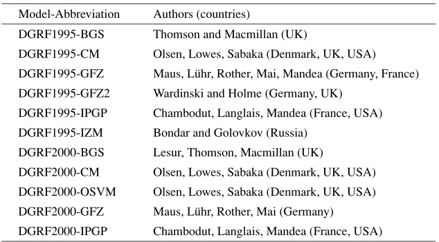
Fig. 1. Differences inX,YandZcomponenets from IGRF and DGRF models for epoch 1995.0. The countour interval is 50 nT.

|d Dst(t)/dt| ≤3 nT/hour and only measurements made in thereal shadow sideof the Earth (Chambodutet al., 2003).

Modelling method For the inversion process data were randomly selected (10 data per 3◦ ×3◦ equiangular bin). A geographic weighting scheme was applied on satellite datasets and the anisotropy of star camera accuracy con-sidered (Holme, 2000). A undamped iterative least squares routine was used, with the internal terms computed up to

Ni =29 andNSV =10, the external terms toNe=2, with

Dstdependence for degree 1.

Using this first model all data were tested, and outly-ing data removed (for residual larger than 5 nT). Again, the remaining data were randomly selected, as in the ini-tial model, and a new model computed with Ni = 20 and

-30

-30

0 0

0

0

0

0

0

0

0

0 0

10

10

10

10

-20

-20

0

0

0

0

0

0 0

0

0

0 0

0

10 10

10

10

10 10

10 10

10

0

0

0 0

0

0 0

0 0

0

0

0 10

10

10 10

10

10

10

10 ₁₀

10

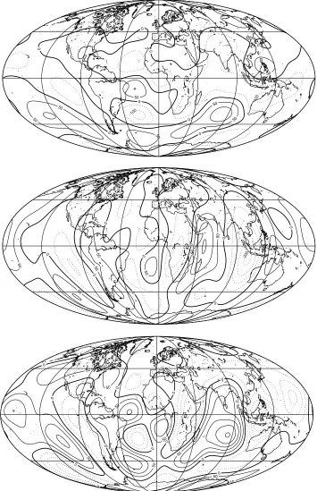
Fig. 2. Differences inX,YandZcomponenets from IGRF and DGRF models for epoch 2000.0. The contour interval is 10 nT. The DGRF2000 model was considered up to degree/order 10, as was the IGRF2000.

4.

Conclusions

The aim of working group V-MOD of the IAGA Divi-sion V is to promote and coordinate international efforts to model and analyze the internal geomagnetic field and its secular variation on both global and regional scales. This is an ongoing process as the current predictive IGRF is re-placed with more accurate DGRF models while new pre-dictive models are adopted for the next 5-years. To illus-trate the continuing need for update, the adopted IGRFs

de-gree/order 10. The differences observed for 1995.0 epochs are, generally speaking, one order of magnitude larger then those for 2000.0.

For the 1995.0 epoch some very large differences (hun-dreds of nT) occur, predominantly in the Southern Hemi-sphere and in the Z component. This is mainly due to the uneven distribution and reduced number of available data used in developing the 8th generation IGRF. The Ørsted satellite brought significant improvements in data coverage, and in the new IGRF models. As a result of the improved data quality and coverage, higher degree and order spher-ical harmonics are now feasible. We believe that the new modelling techniques and the forthcoming missions, such asSwarm(Friis-Christensenet al., 2004) will dramatically improve our field knowledge, as well as the IGRF/DGRF models.

Acknowledgments. My personal thanks for the support received from various organizations and individuals in the international ef-forts to produced IGRF/DGRF models. I would like to thank Su-san McLean, Tatiana Bondar and the guest editor SuSu-san Macmil-lan for useful suggestions that helped in improving the paper. All maps were plotted using the GMT software (Wessel and Smith, 1998). This is IPGP contribution 2055.

References

Cain, J. C., S. J. Hendricks, R. A. Langel, and W. V. Hudson, A proposed model for the International Geomagnetic Reference Field 1965,J. Geo-mag. Geoelectr.,19, 335–355, 1967.

Chambodut, A., J. Schwarte, B. Langlais, H. L¨uhr, and M. Mandea, The selection of data in field modeling,Proceedings 4th OIST (Ørsted Inter-national Science Team conference) meeting, 31–34, 2003.

Chambodut, A., B. Langlais, and M. Mandea, Candidate main-field models for the Definitive Geomagnetic Reference Field 1995.0 and 2000.0,

Earth Planets Space,57, this issue, 1197–1202, 2005.

Friis-Christensen, E., A. De Santis, A. Jackson, G. Hulot, A. Kuvshinov, H. L¨uhr, M. Mandea, S. Maus, N. Olsen, M. Purucker, M. Rothacher, T. Sabaka, A. Thomson, S. Vennerstrom, and P. Visser,Swarm. The Earth’s Magnetic Field and Environment Explorers, ESA SP-1279(6), 2004. Holme, R., Modelling of attitude error in vector magnetic data: application

to Oersted data,Earth Planets Space,52, 1189–1197, 2000.

Langlais, B. and M. Mandea, An IGRF candidate main geomagnetic field model for epoch 2000 and a secular variation model for 2000–2005,

Earth Planets Space,52, 1137–1148, 2000.

Olsen, N., A model of the geomagnetic field and its secular variation for epoch 2000,Geophys. J. Int.,149, 454–462, 2002.

Olsen, N., F. Lowes, and T. J. Sabaka, Ionospheric and induced field leak-age in geomagnetic field models, and derivation of candidate models for DGRF 1995 and DGRF 2000,Earth Planets Space,57, this issue, 1191–1196, 2005.

Sabaka, T., N. Olsen, and R. A. Langel, A comprehensive model of the quiet-time, near-Earth magnetic field: phase 3,Geophys. J. Int.,151, 32–68, 2002.

Sabaka, T., N. Olsen, and M. E. Purucker, Extending comprehensive mod-els of the Earth’s magnetic field with Ørsted and CHAMP data, Geo-phys. J. Int.,159, 521–547, 2004.

Wessel, P. and W. H. F. Smith, New, improved version of the Generic Mapping Tools released,EOS Trans. AGU,79, 579, 1998.