R E S E A R C H
Open Access
Learning of robust spectral graph
dictionaries for distributed processing
Dorina Thanou
1*and Pascal Frossard
2Abstract
We consider the problem of distributed representation of signals in sensor networks, where sensors exchange quantized information with their neighbors. The signals of interest are assumed to have a sparse representation with spectral graph dictionaries. We further model the spectral dictionaries as polynomials of the graph Laplacian operator. We first study the impact of the quantization noise in the distributed computation of matrix-vector multiplications, such as the forward and the adjoint operator, which are used in many classical signal processing tasks. It occurs that the performance is clearly penalized by the quantization noise, whose impact directly depends on the structure of the spectral graph dictionary. Next, we focus on the problem of sparse signal representation and propose an algorithm to learn polynomial graph dictionaries that are both adapted to the graph signals of interest and robust to quantization noise. Simulation results show that the learned dictionaries are efficient in processing graph signals in sensor networks where bandwidth constraints impose quantization of the messages exchanged in the network.
Keywords: Distributed processing, Graph signal processing, Quantization, Polynomial dictionaries, Sparse approximation
1 Introduction
Wireless sensor networks have been widely used for applications such as surveillance, weather monitoring, or automatic control, that often involve distributed signal processing methods. Such methods are typically designed by assuming local inter-sensor communication, i.e., com-munication between neighbor sensors, in order to achieve a global objective over the network. While in theory the performance depends mainly on the sensor network topology, it is largely connected to the power or commu-nication constraints and limited precision operations in practical systems. In general, the information exchanged by the sensors has to be quantized prior to transmis-sion due to limited communication bandwidth and limited computational power. This quantization process may lead to significant performance degradation, if the system is not designed to handle it properly.
In distributed settings, the set of sensors is generally represented by the vertices of a graph, whose edge weights capture the pairwise relationships between the vertices. A graph signal is defined as a function that assigns a real
*Correspondence:[email protected]
1Swiss Data Science Center, EPFL, Lausanne, Switzerland Full list of author information is available at the end of the article
value to each vertex, which corresponds to the quantity measured by the sensor, such as the current tempera-ture or the road traffic level at a particular time instance. Graph dictionary representations are certainly powerful and promising tools for representing graph signals [1]. In particular, when graph signals mostly capture the effect of a few processes on a graph topology, the graph signals can be modeled as the linear combinations of a small number of constitutive components in a spectral graph dictionary [2,3]. Such dictionaries, which can also be seen as a set of spectral filters on graphs, incorporate the intrinsic geo-metric structure of the irregular graph domain into the atoms and are able to capture different processes evolv-ing on the graph. Moreover, they can exhibit a polynomial structure [3] or can be approximated by polynomials of a graph matrix [4, 5] (e.g., spectral graph wavelets). As such, they can be implemented distributively and there-fore represent ideal operators for graph signal processing in sensor networks1.
The distributed processing of graph signals in sensor networks from a graph signal representation perspec-tive has received a considerable amount of attention recently. The works in [4, 5] study how a general class of linear graph operators can be approximated by shifted
Chebyshev polynomials and can eventually be applied to distributed processing tasks such as smoothing, denois-ing, and semi-supervised classification. A distributed least square reconstruction algorithm of bandlimited graph sig-nals has been proposed in [6], and a distributed inpainting algorithm for smooth graph signals was introduced in [7]. The finite-time behavior of distributed algorithms on arbitrary graphs is studied in [8], showing that any arbitrary initial condition after many distributed linear iterations can be forced to lie on a specific subspace. More recently, distributed strategies for adaptive learning of bandlimited graph signals from a probabilistic sam-pling point of view were developed in [9]. The works of [10–12] study the design of graph filters, i.e., distributed linear operators for in the context of graph signal process-ing, with [11,12] focusing specifically on ARMA and IIR filters, respectively. However, neither of these works takes into consideration the effect of the quantization noise that is of significant importance in realistic sensor net-work scenarios with rate and communication constraints. Limited attention to the effect of quantization is given in [13,14], in the context of linear prediction with graph fil-ters. However, the focus of those works is the design of generic graph filters without taking into account the effect of quantization in the design itself. The effect of quantiza-tion in the design of distributed representaquantiza-tions for graph signals has been studied in our preliminary work [15], and more recently in [16]. The latter however focuses on the approximation of the frequency response of known graph FIR filters with filters that are robust to quantization noise, rather than the distributed processing of the graph signals. In this paper, we build on our previous work [15], and we study the effect of quantization in distributed graph signal representations. In particular, we first derive the quantization error that appears in the distributed com-putation of different operators defined on graph spectral dictionaries with polynomial structures. Our analysis is quite generic and can be applied to every graph spectral dictionary that can be approximated by polynomials of the graph Laplacian (e.g., spectral graph wavelets approx-imated with Chebyshev polynomials) [4, 5]. We then consider the problem of sparse representation of graph signals that is implemented in a distributed way with an iterative soft thresholding algorithm. We analyze the convergence of the algorithm and show how it depends on the quantization noise, whose influence is itself gov-erned by the characteristics of the dictionary. We finally propose an algorithm for learning polynomial graph dic-tionaries that permits to control the robustness of dis-tributed algorithms to quantization noise. Experimental results illustrate the dictionary design trade-offs between accurate signal representation and robustness to quanti-zation errors. They show in particular that it is necessary to sacrifice on signal approximation performance for
ensuring proper convergence of distributed algorithms in low-bit rate settings. To the best of our knowledge, the work done in this paper is definitely one of the first steps toward designing quantization-aware dictionaries for distributed signal processing.
The rest of the paper is organized as follows. In Section 2, we model the sensor network with a graph, and we recall the use of polynomial graph dictionaries for distributed processing of graph signals. We study the quantization error that appears in the distributed compu-tations with polynomial graph dictionaries in Section3, and in Section4, we analyze the specific case of the sparse approximation of graph signals. In Section5, we propose an algorithm for learning polynomial graph dictionaries that are robust to quantization noise. Finally, in Section6, we evaluate the performance of our algorithm in both synthetic and real world signals.
2 Polynomial graph dictionaries for distributed signal representation
For the sake of completeness, we recall some of the basic concepts of signal representation on graphs, and we introduce notations that are needed for the rest of this paper. First, we model the sensor network topology as a weighted graph, whose connectivity defines the commu-nication channels. Moreover, we recall briefly the sparse signal model that is based on polynomial dictionaries of the graph Laplacian. Such dictionaries lead to efficient distributed computations, as illustrated in what follows.
2.1 Notation
Throughout the paper, lowercase normal (e.g., a), low-ercase bold (e.g., x), and uppercase bold (e.g., D) letters denote scalars, vectors, and matrices, respectively. Unless otherwise stated, calligraphic capital letters (e.g.,V) rep-resent sets.
2.2 Distributed sensor network topology
We consider a sensor network topology that is modeled as a weighted, undirected graph G = (V,E,W), where V ∈ {1,. . .,N} represents the set of sensor nodes and
N = |V|denotes the number of nodes. An edge denoted by an unordered pair{i,j} ∈E represents a communica-tion link between two sensor nodesiandj. Moreover, a positive weightWij>0 is assigned to each edge{i,j} ∈E. D is a diagonal degree matrix that contains as elements the sum of each row of the matrixW. The set of neigh-bors for nodeiis finally denoted asNi= {j|{i,j} ∈E}. The normalized graph Laplacian operator is finally defined as L= I−D−12WD−12. We denote its eigenvectors byχ =
χ1,χ2, ...,χN
, and the spectrum of the eigenvalues by:
The eigenvalues of the graph Laplacian provide a notion of frequency on the graph and the corresponding eigen-vectors define the graph Fourier transform [1]. In par-ticular, for any functionydefined on the vertices of the graph, the graph Fourier transformyˆ at frequency λ is defined as:
ˆ
y(λ)= y,χ = N
n=1
y(n)χ∗(n),
while the inverse graph Fourier transform is obtained by projecting back in the (orthonormal) graph Fourier basis.
We note that the underlying assumption of this work is that the structure of the signal is captured by the com-munication graph. This assumption is generally true in sensor network applications, where the communication is restricted to neighboring sensors. As an example, the transportation graph is expected to have a strong influ-ence on the traffic sensor measurements. The communi-cation graph in that case can be considered as a proxy for the transportation graph.
2.3 Sparse graph signal model
We model the sensor signals as sparse linear combina-tions of (overlapping) graph patternsg(·), positioned at different vertices [3]. Each pattern defined in the graph spectral domain captures the form of the graph signal in the neighborhood of a vertex, and it can be considered as a function whose values depend on the local connectivity around that vertex. We represent the translation of such a pattern to different vertices of the graph [17] through a graph operator defined as:
g(L)=χg()χT. (1)
The generating kernelg(·), which is a function of the eigenvalues of the Laplacian, characterizes the graph pat-tern in the spectral domain. One can design graph oper-ators consisting of localized atoms in the vertex domain by taking the kernelg(·)in (1) to be a smooth polynomial function of degreeK[3,17]:
g(λ)= K
k=0
αkλk, =0, ...,N−1. (2)
A graph dictionary is then defined as a concatenation of subdictionaries in the formD = g1(L),g2(L), ...,gS(L)
, where each subdictionarysis defined as:
gs(L)=χ K
k=0
αskk χT = K
k=0
αskLk. (3)
A subdictionaryg(L) corresponds to a matrix, each col-umn of which is an atom positioned at a different vertex of the graph. For the sake of simplicity, we assume that
all the subdictionaries are of the same order K. How-ever, all the results presented in the manuscript hold for subdictionaries with different polynomial degrees.
Finally, a graph signalycan be expressed as a linear com-bination of a set of atoms generated from different graph kernelsgs(·)
s=1,2,...,S,
y= S
s=1
gs(L)xs= S
s=1 Dsxs,
where we have setDs = gs(L) ∈ RN×N, andxs ∈ RN are the coefficients in the linear combination. One can then learn the polynomial coefficients numerically from a set of training signals that live on the graph as shown in [3] in order to adapt the dictionary to specific classes of signals. Another example of the dictionary D is the spectral graph wavelet dictionary [17] with pre-defined spline coefficients, or more generally the union of graph Fourier multipliers that can be efficiently approximated with Chebyshev polynomials [5].
2.4 Distributed computation of the graph operators An important benefit of polynomial graph dictionaries described above is the fact that they can be efficiently stored and implemented in distributed signal process-ing tasks. Each polynomial dictionary can be constructed locally, i.e., by exchanging only information between nodes that are connected by an edge on the graph. For the sake of completeness, we recall here the distributed com-putation of some of these operators. More details can be found in [4].
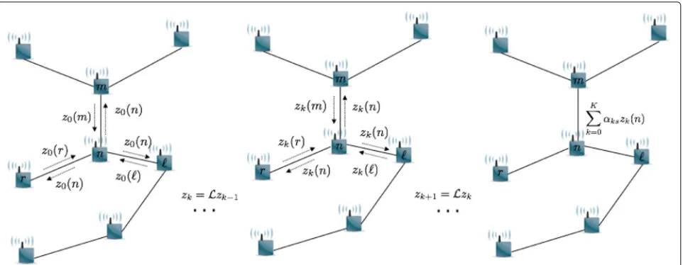
The distributed computation ofDTyrequires first the computation of the different powers of the Laplacian matrix, i.e., L0y,L1y,L2y, ...,LKy, in a distributed way. The latter can be done efficiently by successive multipli-cations of the matrixLwith the signalyoverKiterations. We introduce a new variablezk ∈RN in the computation of DTy, which represents the value transmitted during thekthiteration, withz0 = y. Initially, each node trans-mits its component ofz0only to its one-hop neighbors on the graph. After receiving the values from its neighbors, it updates its component as a linear combination of its own value inz0and the values received from its neighbors as follows:
z1=Lz0. (4)
At the next iteration, the values of z1 are exchanged locally in the network. The procedure is repeated over
K iterations, and the exchanged messages are computed based on the previous recursive update relationship. After knowing {z0(n),z1(n), ...,zK(n)}, each node n can com-pute thenthcomponent ofD
Fig. 1Distributed computation ofDsyin a sensor network. Sensornexchanges messages with its one-hop neighbors forKiterations. After each iteration, the received messages are filtered with weights defined by the graph Laplacian, i.e.,zk(n)=(Lzk−1)(n), and are transmitted locally in the network.(Dsy)(n)is computed as a linear combination of the messages exchanged during theKiterations
K
k=1αskzk(n). The same can be done for the differ-ent subdictionaries and their polynomial coefficidiffer-ents. An illustration of the process is shown in Fig. 1. The main steps are given in Algorithm 1.
Algorithm 1Distributed computation ofDTy 1: Input at noden:y(n),Ln,:,α=[α1; ...;αS]
2: Output at noden:(DTy)(s−1)N+nfor all s =
{1, ...,S}
3: Transmitz0(n)=y(n)to all neighbors inNn 4: Receivez0(m)=y(m)from all neighbors inNn 5: fork=2, ...,Kdo:
6: Transmitzk−1(n)=(LTzk−2)(n)to all the neighbors
7: Receivezk−1(m)=(LTzk−2)(m)from all the neighborsm∈Nn.
8: end for
9: ComputezK(n)=(LzK−1)(n) 10: fors= {1, ...,S}do
11: Compute(DTy)(s−1)N+n=Kk=0αkszk(n) 12: end for
Following the same reasoning, the forward operatorDx can be computed in a distributed way. We recall that
Dx = Ss=1Dsxs, wherex = (x1, x2, ... ,xs) ∈ RSN is a vector with the sparse codesxscorresponding to subdic-tionaryDs. Each of the components in the summation is computed by sending iteratively the powers of the Lapla-cian as follows. For each of the subdictionaries, we define a new variable zs,0 = xs. The transmitted value of this variable by sensornat iterationkis:
zs,k(n)=(Lzs,k−1)(n).
Each sensor can then compute its component in Dx, which can be expressed as follows in a vector form:
Dx= S
s=1 Dsxs=
S
s=1 K
k=0
αskzs,k.
The main steps of the distributed algorithm for the com-putation of Dx are shown in Algorithm 2. Finally, the operatorDTDx can be implemented in distributed set-tings by first computingDxand thenDTDxby following Algorithms 2 and 1, respectively.
Algorithm 2Distributed computation ofDx
1: Input at node n: x(s − 1)N + n, for all s =
{1, ...,S},Ln,:,α=[α1; ...;αS] 2: Output at noden:(Dx)(n)
3: Setzs,0(n)=x
(s−1)N+mfor alls= {1, ..,S}. 4: fork=2, ...,Kdo:
5: Transmitzs,k−1(n) = (Lzs,k−2)(n) to all the neigh-bors, for alls= {1, 2, ...,S}.
6: Receive zs,k−1(m) from all m ∈ Nn, for all s = {1, 2, ...,S}.
7: end for
8: Computezs,K(n)=(Lzs,K−1)(n), for alls= {1, ...,S}. 9: Compute and output(Dx)(n)=Ss=1Kk=0αkszs,k(n).
the computation of quantities such as the forward applica-tion of the dicapplica-tionary and its adjoint to be performed only by local exchange of information.
3 Distributed processing with quantization We now study the effect of quantization in distributed sig-nal processing with polynomial dictionaries by modeling the propagation of the quantization error in the different dictionary-based operators.
Given a graph signaly , and the representation of the signal in a polynomial graph dictionaryD, i.e.,y = Dx, we study the computation of three basic operators, i.e., the forward operatorDx, the adjoint operatorDTy, and the operatorDTDxin distributed settings when the sen-sors exchange quantized messages. Although our main focus is on graph dictionaries that are given directly in a polynomial form of the graph Laplacian operator, we note that the following results hold for every graph dictionary that can be approximated by a polynomial of any graph connectivity matrix (e.g., graph shift operator, adjacency matrix). In what follows, we assume that at every iteration, each sensor measurement is quantized with a uniform quantizer whose parameters are defined by the initial sen-sors states. In particular, we define a finite interval of size S = S0(max)−S0(min). The parametersS(0min) andS0(max)
represent the minimum and the maximum values of the interval, respectively, that are defined a priori. In the case of aq-bit uniform quantizer, the parameter = S/2q is the quantization step-size, which drives the error of the quantizer.
3.1 Distributed computation ofDTywith quantization As we already saw in Section 2.4, the distributed computation of DTy requires first the computation of the different powers of the Laplacian matrix, i.e., {L0y,L1y,L2y, ...,LKy}, in a distributed way. The latter can be done efficiently by successive multiplications of the matrixLwith the signalyoverKiterations, which as we will see next contains some noise that is accumulated over the iterations when the messages are quantized. Recall that the variablezk in the computation ofDTycaptures the sensors’ values at thekthiteration, withz0=y. Before the sensors exchange information, the value of this vari-able at sensornand iterationk, i.e.,zk(n), is now quantized such that:
˜
zk(n)=zk(n)+k(n), (5) wherek(n)is the quantization error ink, andz˜k(n)is the quantized value that the sensornsends to its neighbors. In particular, in the case of aq-bit uniform quantizer, the quantized values can be written as:
˜
Then, each node updates the local value of the vari-ablezkas a linear combination of its own quantized value and the quantized values received from its neighborsz˜k(i) withi∈Nn, based on the recursive update relationship in a vectorized form:
zk+1=L(zk+k). (6) By taking into consideration the quantization error from the previous iterations, Eq. (6) can be re-written as:
zk+1=Lk+1z0+ k
l=0
Lk+1−ll. (7)
We observe that the quantization process involved in the transmission of the different powers of the Laplacian induces some quantization noise that is accumulated over theKiterations and is represented by the second term of Eq. (7).
We now compute DTsy, the quantized vector corre-sponding toDTsy, by applying the polynomial coefficients on the values generated by the sequence {z0,z1, ...,zK}
is the overall accumulated quantization noise that occurs in the distributed computation ofDTsy. Finally, the global
operationDTy= DTsyS
s=1in the presence of quantiza-tion can be written as:
RSNthat contains as entries the error obtained by applying theSdifferent sets of polynomial coefficients to the accu-mulated quantization noise. The distributed algorithm for computingDTyis summarized in Algorithm 3.
Algorithm 3Distributed computation ofDTywith to all the neighbors.
9: Receivez˜k−1(m)from all the neighborsm∈Nn.
by sending iteratively the powers of the Laplacian as described in Section2.4. The quantization effect through the iterative process is significant. To elaborate on that, for each of the subdictionaries, we define a new variable zs,0 =xs. The quantized value of this variable at sensorn and iterationkthat sensornsends to its neighbors reads:
˜
zs,k(n)=zs,k(n)+ζs,k(n), (9)
where ζs,k(n) is the quantization error, and zs,k(n) is the value of the sensor before quantization that is computed as:
By taking into consideration the quantization error com-ponents from the previous iterations, the values of the sensors at iterationk+1 are defined as:
zs,k+1=Lk+1zs,0+
where the accumulated quantization noise corresponding to subdictionaryDsis defined as:
E(Dsxs)=
The main steps of the distributed algorithm for the com-putation of Dx with quantized messages are shown in Algorithm 4.
Algorithm 4Distributed computation ofDxwith quantization
3.3 Distributed computation ofDTDxwith quantization Finally, we illustrate the distributed computation of
is defined asz0=Dx. The sensors’ values at iterationk+1
where ξl is the quantization error vector ξl = (ξl(1),ξl(2), ...,ξl(N))that occurs after transmittingz˜l. By
where we have set
E(Dx)= observe that there is an error accumulated from the com-putation of both steps DxandDTDx that depends on the quantization noise and the structure of the dictionary through the coefficients {αsk}Ss=,K1,k=0. The main steps of the algorithm are shown in Algorithm 5.
Algorithm 5 Distributed computation of DTDx with
quantization to all the neighbors.
9: Receivez˜k−1(m)from all the neighborsm∈Nn.
Finally, we note that while the above analysis of the quantization noise is based on the normalized graph Laplacian matrix, it holds for any other graph matrix that captures the communication pattern of the network, such as the combinatorial Laplacian, and the adjacency matrix. In the next section, we give an illustrative exam-ple of the use of such operators in the distributed sparse representation of graph signals.
4 Distributed sparse graph signal regularization with quantization
In the following, we use the above operators for the dis-tributed computation of a sparse representation of a signal ywith respect to a dictionaryD, under communication constraints. The sparse representation in a dictionaryD can be found by solving a LASSO minimization problem [20] as shown next.
4.1 Illustrative application of distributed graph signal processing
We consider the distributed processing scenario where each noden of the graph computes the sparse decom-position in a polynomial dictionary by solving a sparse regularization problem of the form:
x∗=argmin x ||
y−Dx||22+κx1, (14)
sparse prior. We thus start with the underlying assump-tion that the signal y is sparse in a polynomial graph dictionary, whose coefficients are known to all the sen-sors. Moreover, node n knows its own component of a signal y ∈ RN (i.e.,y(n)) and thenth row of the corre-sponding Laplacian matrixLn,:. The above problem can be solved by an iterative soft thresholding algorithm (ISTA) [23], in which the update of the estimated coefficients is given by:
x(t)=Sκτ
x(t−1)+2τDTy−Dx(t−1)
, t=1, 2, ... (15)
where τ is the gradient stepsize, and Sκτ is the soft thresholding operator:
Sκτ(z)= !
0, if|z| ≤κτ z−sgn(z)κτ, otherwise,
which corresponds to the proximal operator of the κx1function. Thus, the whole algorithm is a particular instance of the general family of proximal gradient meth-ods [24]. By combining the distributed computation of the operationsDTy,DTDx, andDx, as described in the pre-vious subsection, each iteration of ISTA can be solved in a distributed way [4]. In particular, in the first iteration, each node nmust compute(Dsy)(n) for all the subdic-tionaries, via Algorithm 1. In each iteration(t+1), it must compute first(Dx(t))(n), and sequentially applyDTDx(t) via Algorithms 2 and 1, respectively. The solution of (14) is found after a stopping criteria is satisfied (e.g., a fixed number of iterations is executed). The estimate of the sig-nal at each node is then given by computingyˆ =Dx∗via Algorithm 2.
The computational complexity for each iteration of ISTA depends mainly on the matrix operations that are involved in the process, i.e., the dictionary forward and adjoint operators. We briefly discuss these steps here. We recall thatDTy=Ss=1Kk=0αskLky. The computational cost of the iterative sparse matrix-vector multiplication required to computeLkyk=0,2,...,K isO(K|E|), where|E| is the cardinality of the edge set of the graph. There-fore, the total computational cost to compute DTy is
O(K|E| +NSK). We further note that, by following a pro-cedure similar to the one in [17], the term DDTycan also be computed in a fast way by exploiting the fact that
DDTy = S
s=1gs2(L)y. This leads to a polynomial of degreeK = 2K that can be efficiently computed. Simi-lar reasoning can be followed to compute the complexity of the other operations involved in the process. SinceS,K
are relatively small, the complexity of ISTA at each itera-tion is mainly dominated by the size of the graph, and the number of edges.
4.2 Performance of ISTA under quantization constraints The first step of ISTA requires the computation of the gra-dient of the fitting term of Eq. (14), i.e.,y−Dx2, which implies the computation of the operationsDTy, DTDx in each iteration of the algorithm. When the messages exchanged by the sensors are quantized, the quantization noise induced by each of these operations introduces an error in the gradient, such that:
˜
x(t)=Sκτ
x(t−1)+2τ
DTy−DTDx(t−1)+e(t−1), (16)
wheree(t−1)is the total gradient error, which according to Eqs. (8), (11), and (13) can be expressed as:
e(t−1)=E(t−1)
DTy−DTE(t−1)(Dx)−E(t−1)DTDx. The convergence of the sparse graph signal representa-tion by the ISTA algorithm then depends on the sequence of errors over the iterations. It can be characterized by the following result from [25] that applies to the general family of proximal gradient methods such as ISTA.
Theorem 1([25])Let f be a differentiable with Lipschitz continuous gradient function on some compact set with Lipschitz constant L, g a lower semi-continuous and con-vex function, and{τt}a sequence of gradient stepsizes that
satisfy the conditions:
0< β≤τt≤min(1, 2/L−β),with0< β < 1
L. Then, the sequence generated by the iterates
x(t)=proxτt−1g
x(t−1)−τt−1∇f
x(t−1)
+τt−1e(t−1)
(17)
converges to a stationary pointx∗if, given a fixedτ¯, the following condition on the gradient error holds:
∀τ ∈(0,τ¯] , τe ≤ ¯, for some¯≥0.
The above result indicates that the proximal gradient method converges to an approximate stationary point if the norm of the gradient error is uniformly bounded. Furthermore, if the number of perturbed gradient com-putations is finite, or if the gradient error norm converges toward 0, then the sequence limit point is the exact solu-tion of the initial problem. Therefore, we have to make sure that the error in the gradient is bounded so that the distributed sparse graph signal representation algorithm converges.
bound on the norm of the error is given by the following lemma.
Lemma 1Let e(t−1) be the error vector due to quan-tization in the computation of the gradient at iteration t−1as defined in Eq. (16) andthe quantization step-size of a uniform quantizer. Then, the quantization error is bounded as:
The proof of Lemma 1 is provided in the “Appendix” section.
The above inequality shows that the error at each iteration of the gradient is upper bounded by the quantization stepsize, multiplied by a matrix polyno-mial of the graph Laplacian L. The quantization errors depend on the number of bits, i.e., the rate con-straints on data exchanged in the sensor network. For a uniform quantizer, the magnitude of the quantization error is upper bounded by the quantization stepsize. In particular, if the norm ###Kj=−1lαs(l+j)Lj### is bounded
Thus, the error of the gradient at each iteration is bounded, which implies that ISTA converges to a station-ary point of the iteration (17) according to Theorem 1. When → 0, i.e., the bit rate tends to infinity, and the quantization noise tends to zero, e(t−1) → 0, inde-pendently of η. However, when the number of bits is limited and fixed, the quantization noise depends on the characteristics of the dictionary. When the norm of the polynomial of the Laplacian matrix goes to zero (i.e., η → 0), the error also tends to 0 (i.e., ##e(t−1)## → 0). Finally, the upper bound on the error due to quanti-zation in Eq. (19) indicates that the higher the degree
K of the polynomial, the more the error tends to be accumulated over the iterations. This is quite intuitive as higher polynomial degree requires more informa-tion to be exchanged between the sensors, at the cost of more propagation of the quantization noise. A large value of K at the same time guarantees that the poly-nomial functions can better approximate the underlying spectral kernels and thus the graph signals. It indicates that there is a trade-off in the design of the dictionary,
between the representation performance of the polyno-mial dictionary and the propagation of the quantization noise.
5 Polynomial dictionary learning with quantization
We use the study of the previous section to include the quantization parameter in the dictionary design, and we introduce an algorithm to learn polynomial dic-tionaries that are robust to quantization noise. Our approach consists in controlling the norm of the total error in each step of the gradient computation when solv-ing ISTA-based algorithms in a distributed way. When the quantization step size and the graph are given, the total error due to quantized communication can be controlled by choosing the proper values for the polynomial coefficients {αsk}Ss=,K1,k=0 such that the gra-dient error stays bounded. From Eq. (18), the poly-nomial coefficients need to be computed in such a way that the spectral norm ###Kj=−1lαs(l+j)Lj###, for l ∈ symmetric, the spectral norm is simply its largest eigen-value. Therefore, constraining the spectral norm becomes equivalent to constraining the eigenvalues of the corre-sponding matrix.
5.1 Dictionary learning algorithm
of the matrix Kj=−1lαs(l+j)Ljforl ∈ {1, ...,K − 1} ands∈ {1, ...,S}.
Formally, the dictionary learning problem can be cast as the following optimization problem:
argmin α∈R(K+1)S,X∈RSN×M
||Y−DX||2F+μα22
subject to xm0≤T0, ∀m∈ {1, ...,M}, Ds=
K
k=0
αskLk,∀s∈ {1, 2, ...,S} (20)
0IDscI, ∀s∈ {1, 2, ...,S} (c− 1)I
S
s=1
Ds(c+ 2)I,
−ηI
K−l
j=1
αs(l+j)LjηI, ∀l∈ {1, ...,K−1},
whereD=[D1,D2,. . .,DS],xmcorresponds to column
mof the coefficient matrixX,T0is the sparsity level of the coefficients of each signal, andIis the identity matrix. The above dictionary learning formulation is inspired by [3], including some additional constraints that take into account the quantization noise. The spectral constraints provide some control over the spectral representation of the atoms and the stability of signal reconstruction with the learned dictionary as discussed in [3]. In particu-lar, they guarantee that the learned kernels are positive, and the obtained dictionary is a frame. The optimization problem (20) is not convex, but it can be approximately solved in a computationally efficient manner by alter-nating between the sparse coding and dictionary update steps. In the first step, we fix the parameters α (and accordingly fix the dictionaryD) and solve the sparse cod-ing step uscod-ing orthogonal matchcod-ing pursuit (OMP) [26]. In the second step, we fix the coefficientsXand update the dictionary by finding the vector of parameters, α, that solves the polynomial coefficient update step using interior point methods [27].
We notice that the parameter η is a design parame-ter that intuitively should decrease when the quantization stepsize increases (See Eq. (19) for a fixed accumulated quantization error##e(t−1)##). In particular, a large quanti-zation stepsize implies that the accumulated quantiquanti-zation error tends to be large. In that case, a small value of η penalizes the propagation of the quantization noise by learning a dictionary that is more robust in distributed settings, at the cost of a reduced flexibility in the search space of the polynomial coefficients. The latter implies a loss in the accurate recovery of the underlying spectral
kernels that generate the true dictionary atoms. A large value of ηgives more flexibility for a solution of (20) to learn a set of polynomial coefficients that are good for approximating the kernels in ideal communication set-tings, without restricting the accumulated quantization noise however. As a result, if the quantization stepsize is small (i.e., the quantization is fine enough),ηcan be cho-sen relatively big, so that it does not affect the solution of the optimization problem (20).
As mentioned in the introduction, the problem of quantization-aware graph signal representations has been recently studied in [16], from the viewpoint of designing robust FIR filters. In particular, a zero-mean Gaussian i.i.d. initial signal is filtered by a graph filter which is built on a graph shift operator, and it results on an output graph sig-nal. Contrary to our work, the desired frequency response of the filter is known, and the main objective is to find an approximation of that response with a robust graph filter that (i) approximates sufficiently well the desired response and (ii) reduces the amount of quantization noise at the output graph signal. In our formulation of (20), our signals are generated from a sparse signal model, whose repre-sentation matrix, i.e., dictionary, consists of a set of graph filters, whose frequency response is not known. Thus, the goal is to find a set of desired filters that can approximate a set of graph signals, given some predefined constrains that penalize the propagation of the quantization noise. Thus, the focus is more on the representation and processing of the signal rather than on the approximation of a desired frequency response of a filter.
5.2 Analysis of the learned dictionary
To quantify the effect of the quantization constraints on the polynomial coefficients, we derive a few representative bounds. In particular, using the fact that the constraints affect the spectrum of the matrix, for l = K − 1, we of the coefficientαsK is defined by the largest eigenvalue λmax.
Following a similar reasoning, forl= K−2, we obtain that:
Finally, using the above developments, we can recur-sively boundαs(K−3). Following similar reasoning, it can be easily derived that:
−η
We note that the above bounds are quite conservative as they are based on the largest eigenvalue of the graph Laplacian. These types of inequalities however show that
by adding the quantization constraints, we restrict the magnitude of the coefficients. The effect of this trade-off is studied numerically in the next section.
6 Results and discussion
We first study the performance of our dictionary learning algorithm for the distributed approximation of synthetic signals. Then, we study the application of the proposed framework in the denoising of real world signals.
6.1 Synthetic signals
6.1.1 Settings
We generate a graph by randomly placingN = 500 ver-tices in the unit square. We set the edge weights based on a thresholded Gaussian kernel function so thatWij =
e−[dist(
i,j)]2
2θ2 if the physical distance dist(i,j) between
ver-ticesiandjis less than or equal toδ, and zero otherwise. We fixθ = 0.04 and δ = 0.09 in our experiments and ensure that the graph is connected. In our first set of experiments, we construct a set of synthetic training sig-nals consisting of localized patterns on the graph, drawn from a dictionary that is a concatenation ofS = 3 sub-dictionaries. Each subdictionary is a polynomial of the graph Laplacian of degree K=15 and captures one of the three constitutive components of our synthetic signal class. We generate the graph signals by linearly combining
T0≤10 random atoms from the dictionary with random coefficients. We then learn a dictionary from a set of 1000 training signals for different values of the parame-terηthat controls the robustness to quantization error in distributed signal processing.
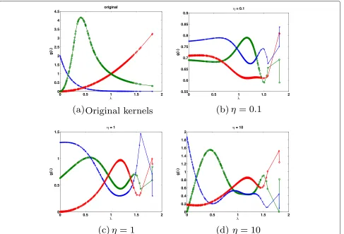
6.1.2 Learned kernels
First, we look in more details on the effect ofη on the dictionary learning outcome and study the effect of this parameter in the learned kernels. In Fig.2a, we illustrate the original kernels of the underlying dictionary, and in Fig.2b–d, we plot the ones recovered by solving the dictio-nary learning algorithm of Eq. (20) for different values of η. As expected, we observe that, as we increase the value of η, the recovered kernels become more similar to the orig-inal ones. The effect of the parameterηis more obvious in Fig.3, where we plot the values of the polynomial coef-ficients. We observe that, whenηis small, the polynomial coefficients become small in magnitude. These results are consistent with the bounds on the polynomial coefficients derived in Section5. In summary, the dictionary learn-ing algorithm is not able to capture relatively complicated kernels, which seems to be the price to pay for improved robustness to quantization.
6.1.3 Approximation performance
Fig. 2Illustration of the kernels recovered for different values ofηin the dictionary learning problem. (a) Original kernels. (b)η=0.1.cη= 1. (d)η= 10
settings without rate constraints. We approximate 1000 testing signals, generated in the same way as the train-ing signals, by computtrain-ing the sparse approximation in the learned dictionaries with OMP, for different sparsity levels. For the sake of comparison, we also compute the approximation performance achieved by applying OMP on the spectral graph wavelet dictionary
[17]. The obtained results are illustrated in Fig.4. Each point in the curve corresponds to the signal to approxima-tion noise ratio (SNR in dB) for different sparsity levels, and it is computed as the average value over all the test-ing signals. As we reduce the values of the parameter η in the dictionary learning algorithm, the approxima-tion performance in the ideal scenario of infinite bit rate
deteriorates significantly. It can become even worse than the one achieved with the spectral graph wavelet dic-tionary, which is not learned to efficiently represent the training signals. This behavior is consistent with the con-clusion drawn from Figs.2and3. The more we reduce the search space (i.e., the smaller the value ofη), the worse is the approximation performance of the graph signals from the learned dictionary.
6.1.4 Distributed approximation performance
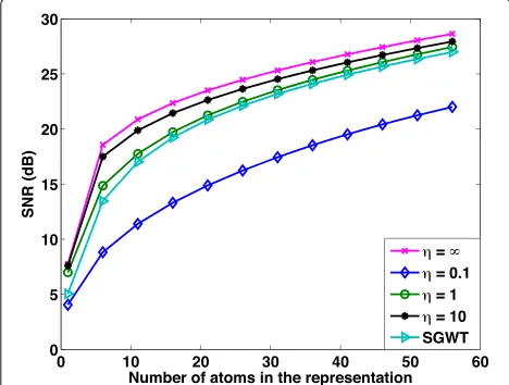
Next, we move to the settings with communication con-straints, and we study the distributed approximation of testing signals using the iterative soft thresholding algo-rithm with iterations defined by Eq. (16). The testing signals are generated in the same way as the training ones. We assume that the messages exchanged by the sensors are uniformly quantized before transmission. In partic-ular, for each message, we send 1 bit for the sign and quantize the magnitude of the data to be transmitted to neighbor sensors. For each signaly, the quantization range of the transmitted messages is defined to be [ 0, y∞], and it is known by all the sensors. We fix the bit rate to 6 bits per message, and we run ISTA for 300 itera-tions and different values of the sparsity parameterκ in Eq. (16). We learn different polynomial dictionaries by solving the optimization problem (20) for different val-ues ofη. For the sake of comparison, we show also the approximation performance obtained with the spectral graph wavelet dictionary approximated by a Chebyshev polynomial of orderK = 30. In Fig. 5, we illustrate the approximation performance in terms of SNR obtained for different numbers of atoms in the representation. The number of atoms is measured by counting the number
Fig. 4Approximation performance (SNR) versus sparsity level, achieved with the polynomial graph dictionary for different values of
ηin centralized settings
Fig. 5Distributed approximation performance (SNR) versus sparsity level, achieved with different polynomial graph dictionary learned with different values ofηin distributed settings, with a bit rate of 6 bits per message
of non-zero elements in the sparse codes for a partic-ular value of κ. Interestingly, we observe that the best representation performance is obtained when η is very small. As we increase the η, the effect of the quanti-zation noise becomes significantly high, which leads to a dramatically low SNR in the distributed approxima-tion algorithm. The worst performance is obtained when η = ∞, which is equivalent to ignoring the robustness constraint in the dictionary learning algorithm. This con-firms that the robustness constraint can indeed reduce the effect of the quantization noise. However, comparing to the performance obtained in the case of infinite bit rate (red curve in Fig.5), we observe a saturation in the maxi-mum SNR that is significantly lower than the one in ideal communication conditions. This is the price to pay for introducing the quantization constraint and reducing the search space in the dictionary learning problem of (20).
6.1.5 Distributed denoising of graph signals
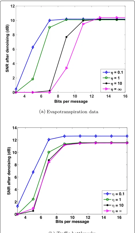
Fig. 6Denoising performance (in dB) versus bits per message using dictionaries learned with different values ofη. The SNR of the input signals is 10 dB
the bit rate is high, the denoising performance obtained with the dictionary corresponding to a smallη(η = 0.1) saturates to a low SNR value. Due to the quantization con-straints, the solution of the optimization problem (20) is not necessarily the optimal one, and the representation performance of the dictionary is reduced. These results are consistent with the ones obtained in the previous experiments.
6.2 Application: denoising of sensor network signals We now consider two real-world datasets, the one con-taining measurements of the evapotranspiration level and the second containing the daily bottlenecks in San Francisco county. The average monthly evapotranspira-tion (ETo) data are recorded at 121 measuring staevapotranspira-tions in California between January 2012 and December 20142. We define a geographical graph, where the nodes of the graph consist of the sensors. Two nodes are connected if the distance between the sensors is smaller than 140 km. The weights of the graph are defined to be inversely proportional to the distance. We compute the average record per month for each station which results in 36 graph signals (i.e., one per month), each of dimension 121. The traffic data are part of the Caltrans Performance Measurement System (PeMS) dataset that provides traf-fic information throughout all major metropolitan areas of California [28]3. It contains signals between January 2007 and August 2014 measured in 75 detector stations. The graph is designed by connecting stations when the distance between them is smaller than a threshold of θ = 0.04. For two stationsAandB, the distancedAB is set to be the Euclidean distance of the GPS coordinates of the stations and the edge weights are computed using the exponential kernels such that WAB = e−dAB. The signal
on the graph is the duration in minutes of bottlenecks for each specific day. We remove the signal instances where no daily bottleneck was identified, and for computational issues, we normalize each signal to a unit norm.
For each of the two datasets, we use the clean signals to learn a polynomial dictionary withS = 3 and maximum polynomial degree ofK = 15. In particular, for the evap-otranspiration data, since the number of available signals is quite limited, we use all the 36 signals for training. The sparsity level is chosen to beT0=30. Regarding the traf-fic data, we use one fourth of the signals for training and the rest for testing. Since these data are in general more sparse, we set the sparsity level toT0 = 5. We run the learning algorithm for different values of the parameter
η =[ 0.1, 1, 10, ∞]. The obtained dictionaries are then used for denoising a set of testing signals in distributed settings, at different bit rates. In the case of the ETo data, the testing signals are generated by adding Gaussian noise of zero mean and variance that depends on the desired SNR to the training signals. For the traffic data, we add Gaussian noise to the testing signals that were not used in the training. The results are illustrated in Figs.7a,b.
First, we observe that under ideal communication, the denoising performance of the evapotranspiration signals is quite poor and the total gain is less than 1 dB. The reason for that is that these data are smoother on the graph, and our polynomial dictionary needs more atoms to approximate them. As a result, a sparse prior in the signals does not necessarily lead to big gains in terms of SNR. On the other hand, the gain observed in the traffic data is higher as such data follows our signal model and consists indeed of localized patterns on the graph. Sim-ilarly to the synthetic data, in both datasets, we observe that we achieve a significant gain when the parameterη is small at low bit rate. On the other hand, as we increase the bit budget, the performance obtained by the uncon-strained dictionary (η= ∞) tends to approximate the one obtained at infinite bit rate.
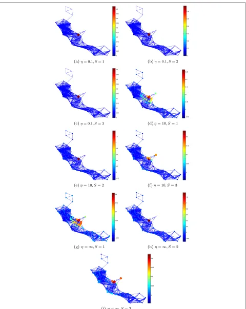
Finally, we study the effect of the parameter η on the learned atoms. For simplicity, we focus only on one dataset. However, similar conclusions can be drawn from the second dataset as well. In Fig. 8, we plot the atoms that are obtained from the traffic dataset and placed at node 10 of the graph. We observe that the smaller the parameterη, i.e., the more we penalize the quantization error, the more localized are the learned atoms. In par-ticular, we observe that all three subdictionaries tend to become similar, which means that the algorithm is learn-ing a dictionary that can be well represented by only one subdictionary. On the other hand, the bigger the parame-terη, i.e., the less we penalize the quantization error, the more the obtained atoms tend to approximate the ones withη = ∞. Thus, they are more spread on the graph. Moreover, each of the subdictionaries tends to capture distinct kernels. These results are quite intuitive and indi-cate that if we want to penalize the quantization noise, we should limit the communication between the nodes of the graph. The latter can be achieved by restricting both the maximum polynomial degree K, i.e., designing simpler and smoother graph kernels, and the number of distinct subdictionariesS, i.e., designing compact dictio-naries with smallS. This, however, comes at the cost of reduced sparsity or worse approximation performance. Since the atoms have a very local support, the number of atoms that is needed to approximate the signal is quite big. As a result, the signals are not very sparse in the obtained dictionary. This may also be a reason for a relatively poor denoising performance of the given dataset.
7 Conclusions
In this paper, we have studied the effect of quantization in distributed graph signal processing with polynomial dictionary operators. We have shown analytically that the overall quantization error depends on the commu-nication pattern of the network captured by the graph Laplacian matrix and the graph structured dictionary. Following this observation, we have then proposed an algorithm that learns polynomial graph dictionaries to sparsely approximate graph signals while staying robust to quantization noise. We have shown that the quantiza-tion constraints penalize the magnitude of the polynomial coefficients, sacrificing on the recovery of the true dic-tionary atoms. Experimental results have illustrated the trade-offs between effective distributed signal representa-tion in low bit rate communicarepresenta-tion settings and accuracy of the signal approximation in ideal settings.
Endnotes
1The main assumption of this paper is that the
com-munication graph coincides with the representation graph that captures that structure of the signals.
2The data are publicly available atwww.cimis.water.ca.gov.
3The data are publicly available athttp://pems.dot.ca.gov.
Appendix
Proof For ease of notation, we ignore the iteration index and we bound the error norm as follows:
e =###EDTy
Similarly, the second and the third terms can be
where the last inequality comes from the assumption that 0I Ds cI, which is a necessary assumption (see the optimization problem 20) for the class of spectral graph dictionaries that we are considering. Combining Eqs. (26)–(29), and using the assumption that the quan-tization noise is uniformly distributed with magnitude smaller than/2, we obtain the upper bound of (18).
Acknowledgements
The authors would like to thank the anonymous reviewers for their constructive comments.
Authors’ contributions
Both authors read and approved the final manuscript.
Competing interests
The authors declare that they have no competing interests.
Publisher’s Note
Springer Nature remains neutral with regard to jurisdictional claims in published maps and institutional affiliations.
Author details
1Swiss Data Science Center, EPFL, Lausanne, Switzerland.2Signal Processing
Laboratory (LTS4), EPFL, Lausanne, Switzerland.
Received: 1 February 2018 Accepted: 14 September 2018
References
1. D.I. Shuman, S.K. Narang, P. Frossard, A. Ortega, P. Vandergheynst, The emerging field of signal processing on graphs: extending
high-dimensional data analysis to networks and other irregular domains. IEEE Signal Process. Mag.30(3), 83–98 (2013)
2. X. Zhang, X. Dong, P. Frossard, inProc. IEEE Int. Conf. Acoustics, Speech, and Signal Process. Learning of structured graph dictionaries, (Kyoto, 2012), pp. 3373–3376
3. D. Thanou, D.I. Shuman, P. Frossard, Learning parametric dictionaries for signals on graphs. IEEE Trans. Signal Process.62(15), 3849–3862 (2014)
4. D.I. Shuman, P. Vandergheynst, P. Frossard, inProc. IEEE Int. Conf. Distr. Comput. Sensor Sys. Chebyshev polynomial approximation for distributed signal processing, (Barcelona, 2011), pp. 1–8
5. D.I. Shuman, P. Vandergheynst, P. Frossard, Distributed signal processing via Chebyshev polynomial approximation. arXiv:1111.5239 (2011) 6. X. Wang, M. Wang, Y. Gu, A distributed tracking algorithm for
reconstruction of graph signals. IEEE J. Sel. Top. Signal Proc.9(4), 728–740 (2015)
7. S. Chen, A. Sandryhaila, J. Kovacevic, inProc. IEEE Int. Conf. Acoustics, Speech, and Signal Process. Distributed algorithm for graph signal inpainting, (Brisbane, 2015), pp. 3731–3735
8. S. Safavi, U.A. Khan, Revisiting finite-time distributed algorithms via successive nulling of eigenvalues. IEEE Signal Proc. Lett.22(1), 54–57 (2015)
9. P.D. Lorenzo, M.P. Banelli, S. Barbarossa, S. Sardellitti, Distributed adaptive learning of graph signals. IEEE Trans. Signal Process.65(16), 4193–4208 (2017)
10. M.S. Segarra, A.G. Marques, A. Ribeiro, Optimal graph-filter design and applications to distributed linear network operators. IEEE Trans. Signal Proc.65(15), 4117–4131 (2017)
11. E. Isufi, A. Loukas, A. Simonetto, G. Leus, Autoregressive moving average graph filtering. IEEE Trans. Signal Proc.65(2), 274–288 (2017)
12. X. Shi, H. Feng, M. Zhai, T. Yang, B. Hu, Revisiting finite-time distributed algorithms via successive nulling of eigenvalues. IEEE Signal Proc. Lett. 22(8), 1113–1117 (2015)
13. A. Sandryhaila, J.M.F. Moura, Discrete signal processing on graphs. IEEE Trans. Signal Proc.61(7), 1644–1656 (2013)
14. J. Liu, E. Isufi, G. Leus, Filter design for autoregressive moving average graph filters. arXiv:1711.09086 (2018)
15. D. Thanou, P. Frossard, inAnnual Allerton Conf. on Communic., Contr., and Comput. Distributed signal processing with graph spectral dictionaries (IEEE, Monticello, 2015), pp. 1391–1398
16. L.F.O. Chamon, A. Ribeiro, inProc. IEEE Glob. Conf. Signal and Inform. Process. Finite-precision effects on graph filters, (Monteral, 2017) 17. D. Hammond, P. Vandergheynst, R. Gribonval, Wavelets on graphs via
spectral graph theory. Appl. Comput. Harmon. Anal.30(2), 129–150 (2010) 18. D.I. Shuman, M.J. Faraji, P. Vandergheynst, inProc. of the Int. Conf. on
Sampling Theory and Applications. Semi-supervised learning with spectral graph wavelets, (Singapore, 2011)
19. S. Segarra, A.G. Marques, G. Leus, A. Ribeiro, Reconstruction of graph signals through percolation from seeding nodes. IEEE Trans. Signal Proc. 64(16), 4363–4378 (2016)
20. S. Chen, D. Donoho, M. Saunders, Atomic decomposition by basis pursuit. SIAM J. Sci. Comput.20(1), 33–61 (1999)
21. R. Tibshirani, Regression shrinkage and selection via the lasso. J. Royal Stat. Society Ser. B.58, 267–288 (1994)
22. S. Chen, D. Donoho, M. Saunders, Atomic decomposition by basis pursuit. SIAM Rev.43(1), 129–159 (2001)
23. A. Beck, M. Teboulle,A fast iterative shrinkage-thresholding algorithm for linear inverse problems. Springer Optimization and Its Applications, vol 49. (Springer, New York, 2009), pp. 183–202
24. P. Combettes, J.C. Pesquet, Proximal splitting methods in signal processing. Fixed-Point Algorithms for Inverse Problems in Science and Engineering, 185–212 (2011)
25. S. Sra, inAdv. Neural Inf. Process. Syst. Scalable nonconvex inexact proximal splitting, (Lake Tahoe, 2012), pp. 530–538
26. J.A. Tropp, Greed is good: algorithmic results for sparse approximation. IEEE Trans. Inform. Theory.50(10), 2231–2242 (2004)
27. S. Boyd, L. Vandenberghe,Convex optimization. (Cambridge University Press, New York, 2004)