Blind sequential detection for sparse ISI channels

R E S E A R C H

Open Access

Blind sequential detection for sparse ISI

channels

Weiwei Zhou

and Jill K. Nelson

Abstract

We present a computationally efficient blind sequential detection method for data transmitted over a sparse intersymbol interference channel. Unlike blind sequential detection methods designed for general channels, the proposed method exploits the channel sparsity by using estimated channel sparsity to assist in the detection of the transmitted sequence. A Gaussian mixture model is used to describe sparse channels, and two tree-search strategies are applied to estimate the channel sparsity and the transmitted sequence, respectively. To demonstrate the performance improvement achieved by the proposed blind detector, we compare it to conventional joint channel and sequence detection methods that use sparse channel estimation techniques. Simulation results show that the proposed detector not only reduces computational complexity compared to existing methods but also provides superior performance, particularly when the signal to noise ratio is low.

Keywords: Blind sequence detection, Sparse channels, Intersymbol interference, Matching pursuit, Tree search

1 Introduction

Intersymbol interference (ISI) poses a great challenge for reliable high-speed wireless communications, signif-icantly degrading system performance, and hence chan-nel equalization is typically employed at the receiver to mitigate its harmful effects. Due to the wide variety of physical conditions that induce frequency selectivity, wireless channels are often unknown and time-varying, thus posing an additional challenge to the receiver. One approach to combating time-varying distortion is via adaptive equalizers [1] that first use training symbols to estimate the channel and then perform conventional detection using the channel estimate. Transmitting a training sequence consumes bandwidth that could oth-erwise be used for transmission of information, however, and training sequences must be transmitted at regular intervals when the channel is time varying.

In order to improve spectral efficiency, considerable research effort has been devoted to the application of blind equalization techniques in wireless communication systems in recent decades [2–8]. A popular approach to blind equalization is to jointly estimate the unknown

*Correspondence: [email protected]

2_{Department of Electrical and Computer Engineering, George Mason}

University, 4400 University Dr., Fairfax, VA 22030, USA

Full list of author information is available at the end of the article

channel and transmitted data based on the maximum likelihood (ML) criterion [9]. The joint estimates are obtained using the least-squares (LS) algorithm for chan-nel estimation and the Viterbi algorithm (VA) for data detection. The LS algorithm is applied iteratively using the data along each surviving path of the VA trel-lis, generating channel estimates that are used in the search extending from each path. One major drawback of joint estimation methods is their potentially prohibitive complexity, particularly for long channels and/or large symbol alphabets. In order to simplify the blind equal-ization process, researchers have proposed blind sequen-tial detection approaches that avoid explicit estimation of the channel [10, 11]. In [10], for example, a frame-work is developed for applying a blind Bayesian maxi-mum likelihood (ML) sequence detector for ISI channels. The channel taps are modeled as stochastic quantities drawn from a known probability distribution, and the tree-based stack algorithm is used to estimate the trans-mitted sequence based on a Bayesian probability met-ric that incorporates implicit estimation of the channel. While the Bayesian ML method achieves promising per-formance results for moderate channel lengths, computa-tional complexity continues to be a drawback for longer channels.

Most existing blind equalization approaches have been designed to recover data transmitted over general (non-sparse) ISI channels. In high-speed wireless applications such as underwater acoustic (UWA) communications, ultrawide band (UWB) communications, and high-definition television (HDTV) systems, the discrete-time channel impulse response has a very large channel mem-ory, but only a small number of significant channel coef-ficients contribute to the distortion of the transmitted signal. When blind equalization approaches that have been designed for general channels are applied to sparse channels, all channel coefficients are treated as significant when estimating the transmitted signal, yielding high-computational burden for the receiver and decreasing the accuracy of the resulting data detection. If we take chan-nel sparsity into consideration when designing the blind equalizer, both computational efficiency and performance can be improved.

In order to blindly estimate a sequence transmitted over a sparse channel, popular sparse channel estimation meth-ods such as matching pursuit (MP), orthogonal matching pursuit (OMP), and basis pursuit (BP) [12–14] can be combined with the VA or stack algorithm using a joint channel estimation and data detection framework. As we show in Section 5, however, these conventional meth-ods result in high complexity, particularly when signal to noise ratio (SNR) is low. In this paper, we propose a com-putationally efficient blind sequential detection method for recovering data transmitted over sparse ISI channels. Two tree-search-based algorithms are used in the blind detection process: the breadth-first M-algorithm (MA) is used to estimate channel sparsity, and the best-first stack algorithm (SA) exploits the channel sparsity esti-mate to efficiently detect the transmitted sequence. The two algorithms use different strategies to search a tree structure. The MA extends all possible paths and retains the M paths with the highest likelihood at a given depth, while the SA extends only the path with the highest likelihood but retains unextended paths. The proposed method moves beyond existing blind sequential detec-tion approaches by incorporating a statistical model of the sparse channel characteristics to reduce the number of path explorations required in the tree search. By combin-ing the two tree-search algorithms in an iterative frame-work, we avoid the need for training data. Additionally, simulations show that computational complexity savings can be achieved when tree-search algorithms are used in place of conventional MP, OMP, and BP for sparse channel estimation.

The remainder of the paper is organized as follows. In Section 2, the overall system model is described, and the sparse channel model is presented. Section 3 provides an overview of the stack-based sequential detection method for unknown sparse ISI channels. The proposed blind

sequential detection algorithm, which combines stack-based sequential detection with channel sparsity estima-tion using the MA, is described in Secestima-tion 4. In Secestima-tion 5, the proposed approach is compared to conventional joint channel estimation and data detection methods that use MP, OMP, and BP with respect to both performance and computational complexity. Section 6 concludes the paper.

2 System model

We consider a discrete-time, baseband equivalent com-munication system, a block diagram of which is shown in Fig. 1. The information bits are passed through an error control encoder with rateR= 1_r. No training sequence is transmitted. For a block of information bits with lengthN, denoted bybN₁, a length-rN sequence of coded bits,xrN₁ , is generated. The encoded sequence is transmitted over a length-Lh sparse ISI channel h =[h0,. . .,hLh−1] with additive white Gaussian noise (AWGN)wkof varianceσ2. The received sequence yrN₁ =[y1,. . .,yrN]T is the input to a detector that blindly estimates the transmitted infor-mation bitsbN₁, where the received signal at time instant k,yk,k=1, 2,. . .,rN, is defined as

yk = Lh−1

i=0

hixk−i+wk. (1)

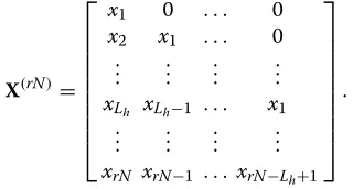
The length-rN received sequence can be expressed in matrix form asyrN₁ =X(rN)h+w, where the signal matrix X(rN)is defined as

X(rN)= ⎡ ⎢ ⎢ ⎢ ⎢ ⎢ ⎢ ⎢ ⎢ ⎣

x1 0 . . . 0 x2 x1 . . . 0

..

. ... ... ... xLh xLh−1 . . . x1

..

. ... ... ... xrN xrN−1 . . .xrN−Lh+1

⎤ ⎥ ⎥ ⎥ ⎥ ⎥ ⎥ ⎥ ⎥ ⎦

.

We assume that the channel has onlyLa active (non-zero) taps, h¯a =[h0,h1,. . .,hLa−1]T, where La Lh. In order to better describe the channel sparsity, we use di ∈ {0, 1}as an indicator to denote whether thei-th tap,

hi, is active or inactive:

di = 0,_1, hiis inactive,

hiis active. (2)

Hence, d = {d0,. . .,dLh−1} is a binary vector that denotes the sparsity of the channel. We assume thatdiis equally likely to be 0 and 1. The number of active channel taps,La, therefore, can be expressed asLa= ||d||0, where thel0-norm of the vectordcounts the number of non-zero elements ind.

Fig. 1System model for sparse ISI channel with blind sequential detector. The databkis passed through an error control encoder with rateR=1_r. The coded sequencexkis transmitted over a sparse ISI channel with additive white Gaussian noisewk. The received sequenceykis processed by a blind sequential detector and decoder to detect the transmitted data sequence

non-zero) values. To reflect this, we use a Gaussian mix-ture to describe the channel tap values. Active taps are drawn from a zero-mean Gaussian distribution with rel-atively large variance, while inactive taps are drawn from a zero-mean Gaussian distribution with much smaller variance [15, 16]:

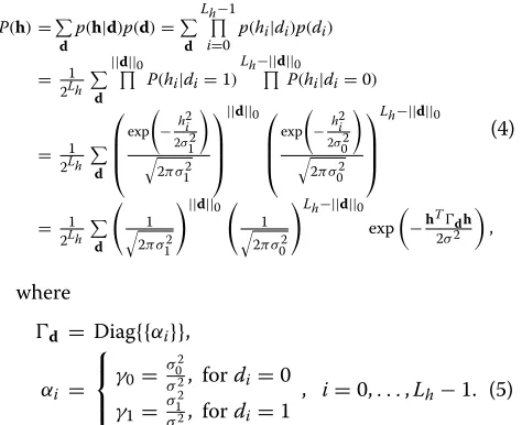
whereσ₀2denotes the variance ofhiin the inactive state, andσ₁2σ₀2denotes the variance ofhiin the active state. We further assume that theLh channel taps are inde-pendent. This assumption is well justified, especially for wireless fading channels that are rich in scattering [17–19]. The distribution of the channelhis then given by

P(h)=

Under this model, the channel is treated as a stochastic random vector at the receiver. The receiver has no knowl-edge of the channel tapshi nor of the sparsity vectord. The diagonal matrixdthat describes the channel sparsity

in (4) varies with realizations of the vectord. The diagonal elementαi=γ1indicates that the channel taphiis active, andαi = γ0indicates thathiis inactive. We assume that the receiver has knowledge of the variance of active and inactive tapsσ₀2andσ₁2. We also assume that the receiver has knowledge of the code generator polynomial C, the variance of the AWGNσ2_{, and the channel lengthL}

h. For simplicity, only binary phase shift keying (BPSK) encoded

data is considered. Extension to transmission of data from larger constellations is straightforward.

3 Stack algorithm for unknown sparse ISI channels

The stack algorithm (SA), which was originally proposed for decoding convolutional and tree codes [20], is a best-first tree-search technique that can be used to approxi-mate the ML solution to sequential detection problems [21]. When the SA is applied to sequential detection, the tree represents the space spanned by a sequence of transmitted bits. Each path in the tree represents a pos-sible realization of the transmitted sequence. A metric is computed for each path; the path metric represents the likelihood that the corresponding bit sequence was trans-mitted, conditioned on the observations. At each time step, the SA extends the path with the highest likelihood (metric) and stores a set of possible paths and their asso-ciated metrics in a stack (or list) in order of decreasing metric value. The SA terminates when the top path in the stack reaches a leaf of the tree, or equivalently when the top path represents a full block of transmitted bits.

To navigate a tree using the SA, paths are progressively extended from depth 1 to depth N. Hence, the algo-rithm must compute the path metric for a partial-length sequence given a full block of observations; this partial-path metric is used to decide which partial-path in the stack will be extended in the next stage. The metric derivation for unknown general ISI channels is introduced in [10]. For sparse ISI channels, we derive a new form for the path metric using the model defined in [10]. The probability that a length-nsequencebn₁=[b1,b2,. . .,bn]T was trans-mitted given the complete received sequenceyrN₁ and the code thus far,C(n)_{, is expressed as} for all paths, and the path metric can be written as

We take the sparsity of the channel into consideration and find a closed-form expression for the integral in (7) using the channel model given in (4). Applying the tech-niques used to derive the path metric for general unknown ISI channels in [10], we assume thatyrn₁ is independent of yrN_rn+1 and that yrN_rn+1 is independent ofbn₁ to obtain the following expression for the path metric:

mbn₁=_2Lh1

Substituting (4) into (8) and integrating the quadratic exponential form yields:

Note that the term

form similar to the least-squares estimate of the channel, demonstrating the implicit learning of the channel vector that is integrated in the metric of the tree-search-based detection approach.

Using the sparse channel model described in Section 2, we are able to incorporate prior information about chan-nel sparsity into the path metric of the SA. However, the computation ofmbn₁in (13) considers all possible real-izations of the vectord. Without simplification, we would need to evaluate and sum 2Lh_{exponential terms, which is} computationally impractical for channels with long delay spread. For a given sparse channel, the sparsity vector d is just one of the 2Lh _{possible binary vectors.} There-fore, if the channel sparsity can be determined, the path metric can be computed for a unique vectord. In order to achieve this, we propose a computationally efficient sparsity estimation technique, described in the following section.

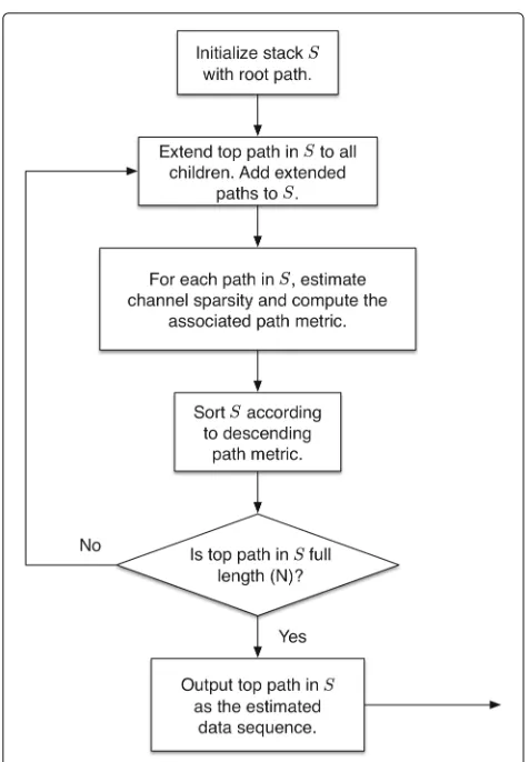
4 Computationally efficient blind sequential detection

4.1 Channel sparsity detection using the M-algorithm The proposed method combines the M-algorithm (MA) and the stack algorithm (SA) to perform blind sequential detection; we refer to the overall algorithm as the MA-SA for simplicity. The MA is used to find the active channel tap indices and estimate the unique binary vectord corre-sponding to the sparse channel. The path metric of the SA is then computed using the channel sparsity estimated by the MA.

Both the MA [22] and the SA are built upon a tree struc-ture representation of the space spanned by a sequence of transmitted bits. In contrast to the SA, however, the MA employs a breadth-first strategy for searching the tree. At a given depth of the tree, it extends all pos-sible paths and retains the M paths with the highest likelihood (or largest path metrics). In the tree struc-ture of the SA, each path represents a possible real-ization of the transmitted sequence; the MA can be used to estimate the channel sparsity along each path. The SA path metrics can be computed using the esti-mated channel sparsity in combination with the obser-vations and the symbol sequence associated with each path. The metrics are used to guide the tree search to find the most likely transmitted sequence. Such a mecha-nism establishes a foundation for combining the MA and the SA. A flow chart of the MA-SA algorithm is shown in Fig. 2.

To better illustrate the proposed algorithm, we pro-vide a step-by-step procedure under the assumption thatM=1.

Step 0. (Initialization) Consider a partial path through the tree that represents a length-n sequencebn₁. The MA-SA algorithm is initialized with the assumption that all channel taps are inactive, i.e.,

Fig. 2A flow chart representation of the MA-SA algorithm

mbn_1d(0)= B(yi) "" "R(rn)

xx +d(0)

"" "−

1 2

2πσ2

0

_Lh

×exp

r(yxrn) T

R(xxrn)+_d(0) −1

r(yxrn)

2σ2

=B(yi)

1

2πσ₀2

Lh

""Rd(0)""−12

×exp

r(yxrn) T

R−1_d(0)_r(rn)

yx 2σ2

,

(15)

where

Rd(0)=R_xx(rn)+_d(0), (16)

and

d(0) =Diag{γ0}. (17)

The vectord(0)is assigned tod(_∗0), where the vectord(∗p)is used to store the best (highest metric) vector obtained at thep-th iteration. A setSis defined to store the associated indices of

the active channel taps at each iteration. Initialize iteration counter top=0and index vector to

S = {}.

Step 1. Change a single 0 element of the binary vector

d(∗p)to 1 to generate a set ofLh−ppossible

binary vectors,d(_jp+1), wherej∈S∈ {1,. . .,L_h}

denotes thatd(_jp+1)is identical tod(∗p)with the exception of thej -th element.

Step 2. Compute the path metricmbn_1d(p+1)

j

for each of

the possible weight-(p+1)vectors, and assign the vector that corresponds to the largest metric to the vectord(_∗p+1), i.e.,d_∗(p+1)=d(_j∗p+1), where

j∗=argmax

j

mbn₁

d(_jp+1), j∈S∈ {1,. . .,Lh}.

(18)

Step 3. Update the index vectorSby includingj∗, and incrementp by 1:

S=S∪j∗, p=p+1. (19)

Step 4. If all active channel tap indices are located or a stopping criterion (described in Section 4.3) is satisfied, terminate the algorithm; otherwise, return to step 1.

The final vector d(Lˆa)

∗ provides the estimate of chan-nel sparsity, whereLˆa denotes the estimate of the active channel length. Lˆa = La if La is known at the receiver. The corresponding metricmbn₁

d(∗Laˆ ) will be used by the

SA to perform the tree search. For a given La, the total number of the metric computations is given by 1+(La+ 1)

Lh− L2a

. We will show in the next section that the number of metric computations can be further reduced. The proposed MA-based sparsity estimation is summa-rized in a flow chart in Fig. 3.

An example of the sparsity estimation procedure is shown in Fig. 4. The example considers a length-4 chan-nel with two active taps,h =[h0, 0,h1, 0], and the figure shows the k-th branch of the SA tree. The red boxes show the best sparsity vectors obtained at each iteration. We initialize the vector d(0) =[0, 0, 0, 0] and compute the path metricmbn_1d(0) using (15). At step 1, there are

four possibilities for the sparsity vector:d(₁1),. . .,d(₄1), and the corresponding path metric can be obtained similar to using (15) for each vector. We assume thatmbn_1d(1)

1 is the

largest path metric at this step, and thusd(∗1) =d(₁1), indi-cating that the first channel tap is active. Fromd(∗1), three possibilities for the sparsity vector,d(₂2),d₃(2), andd(₄2), can be generated. The corresponding path metric for each vec-tor is computed, andmbn_1d(2)

Fig. 3A flow chart representation of the MA-based technique for updating the path metric

Therefore, d(∗2) = d(₃2), indicating that the third chan-nel tap is also active. Now that the two active taps have been located (and assuming the number of active taps is known), the sparsity estimation algorithm can be termi-nated. The quantitymbn_1d(2)

3 serves as the path metric

for the SA at this branch.

4.2 Efficient metric computation

As described in the proposed MA-based sparsity estima-tion, a new path metric is computed at each iteraestima-tion, involving both inversion of a matrix and computing its determinant. The total 1+ (La + 1)

Lh− L₂a

metric computations are still a heavy burden for the detector. By exploiting the properties of matrices, we can further reduce the computational complexity and accelerate the metric update.

In order to develop a general expression for efficient metric computation, consider the binary sparsity vector obtained at the(p− 1)-th iteration: d(∗p−1). The matrix R

d(∗p−1)

in the path metric is computed as

R matrix inversion, the inverse and determinant ofR

d(_ip)

can be easily obtained from the inverse and determi-nant ofR

d(∗p−1)

. We assume that we already have the

inverse and determinant ofR

can then be expressed as

R non-zero element in the vectoruis at indexi. Applying the Sherman-Morrison formula [23], the inverse ofR

d(_ip)

can be expressed as

R−1d(_ip)=Rd(_∗p−1)+βuuT−1 The determinant ofR

d(_ip)

can be computed as

""

Combining Eqs. (23) and (24), the path metric asso-ciated with the sparsity vector d(_ip) can be computed as

mbn1

From (25), we can see that the path metric associated with the vectord(_ip)can be computed via a simple update from the metric ford(∗p−1). The computation for the met-ric update is dominated by the vector multiplications,

r(yxrn)

T

V(:,i)V(i, :)r(yxrn). The inverse and determinant computations are no longer needed at every iteration; they are performed only once to obtain R−1d(0) and

""Rd(0)""when the initial metricmbn_1d(0)is computed.

4.3 Stopping criterion

The MA-based sparsity detection described in Section 4.1 relies on searching for active channel indices and termi-nates when all the active indices have been identified. In practical communication systems, the number of active taps, La, is usually an unknown parameter. A stopping criterion must be implemented to terminate the iterative sparsity detection process without knowledge of La. To address this, we compare the path metrics we obtain at theLa-th and(La+1)-th iterations and use the difference between them to identify a stopping criterion.

mbn₁ exponential function takes a form that is very sim-ilar to the LS estimation of the channel, hˆ. Thus, R(yyrn)[ 0]− errorebetween the received signalyrn₁ and the noise-free output predicted by the channel estimatehˆ and assumed bit sequence xrn₁. At the (La +1)-th iteration, the met-ricmbn_1d(La+1)

∗ associated with the best estimated sparse

vector d(La+1) contribution of the(La+1)-th estimated active tap to the errore, andj∗denotes the index of theLa-th estimated active channel tap.

Assuming that theLa active channel taps are correctly located at theLa-th iteration, no more active taps are con-tributing to the computation of the metric mbn_1d(La+1)

∗ .

Therefore, the corresponding La+1will depend only on additive noise. Given this, we can establish a stopping cri-terion as follows: For a sufficiently small , at the p-th iteration,| p| ≤, the algorithm is terminated. The num-ber of active channel taps can be estimated asLˆa=p−1. The estimated sparse vector isd(∗p−1).

Assuming the algorithm estimates La correctly, one additional round of iterations forp = La+1 is imple-mented (relative to the number of iterations implement whenLais known). This involvesLh−Lametric updates, which is only a small increase in computational com-plexity. When the noise level is high, the algorithm is more likely to estimateLaincorrectly. However, since the channel sparsity is estimated using path metrics that take noise into consideration, we are still able to achieve bet-ter channel sparsity estimation than is achieved using conventional methods, as we show in Section 5.

5 Simulation results and discussion 5.1 Performance comparison

In this section, we compare the proposed method to sev-eral conventional blind sequential detection methods, all of which are based on joint sparse channel estimation and data detection. The method introduced in [24], for example, finds an ML solution for a joint single-input multiple-output channel and sequence estimation prob-lem using a two-step procedure: (1) channel estimates are obtained for every possible data sequence, and (2) the ML data sequence and corresponding channel esti-mate are selected. A least-squares (LS) approach is used to implement step 1, and the VA is used to implement step 2. The LS channel estimation algorithm performs a pseudo-inverse of the channel matrix. When the channel is long but sparse, LS does not provide reliable channel estimation since each tap estimate will have a non-zero value [25]. Additionally, for such channels, the VA is prohibitively complex due to the long-channel memory. Therefore, we use sparse channel estimation techniques such as matching pursuit (MP), orthogonal matching pur-suit (OMP), and basis purpur-suit (BP) to replace the LS approach in the first step. In the second step, we use the SA, which is considerably more efficient than the VA for channels with long delay spread and suffers only minimal performance degradation [26]. The combined methods we consider are denoted by MP-SA, OMP-SA, and BP-SA. In addition to these three methods, we also consider a recently proposed joint sparse channel and sequence detection method using the expectation-maximization (EM) algorithm, SC-EM [27].

The path metric governs the search through the tree to find the most likely transmitted sequence. The tree search continues until a leaf of the tree is reached [31].

The SC-EM algorithm uses a different two-step proce-dure than the three methods described above [27]. The expectation (E) step performs sequential detection using forward-backward recursions (BCJR). ML sparse chan-nel estimation is performed in the maximization (M) step using the estimated sequence of symbols. Iteration between these two steps increases the joint likelihood until convergence is reached.

Simulations have been conducted for a lengthLh = 10 sparse channel withLa = 3 active taps. Information bits are encoded using a rateR = 1₂ convolutional code with generator polynomials g0 =[1, 1, 1] and g1 =[1, 1, 0]. The initial state of the register is set to [0, 0]. Ten thou-sand blocks of 100 data bits each are transmitted over the sparse channel. For each data block, the active chan-nel taps are drawn from a Gaussian distribution with zero mean and varianceσ₁2=1, and the inactive taps are drawn from a Gaussian distribution with zero mean and variance

σ2

0 = 0.01. The channel energy is normalized to 1. The locations of active and inactive channel taps are randomly generated from a discrete uniform distribution for each block. For the three methods, the stack size of the SA is set to 105to make erasures rare. We assume that both the channel response and the number of active channel taps Laare unknown to the receiver.Mis set to 1 when we use MA to estimate the channel sparsity in MA-SA.

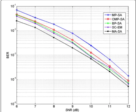
A performance comparison of the five methods described above is shown in Fig. 5. The proposed MA-SA

Fig. 5Performance comparison between MP-SA, OMP-SA, BP-SA, SC-EM, and MA-SA. The performance for each method is computed using 104_{length-100 sequences transmitted over a 10-tap channel} with three active taps

technique outperforms the competing methods, most substantially when SNR is low. This performance gap can be attributed to the fact that MA-SA’s approach of esti-mating the channel sparsity based on the path metric is more robust to noise than are the competing approaches. As expected, OMP-SA yields better performance than MP-SA due to the introduction of the orthogonalization process. MP/OMP do not take the channel noise into consideration and therefore are more likely to incorrectly estimate the sparse channel. Thus, MP-SA and OMP-SA are outperformed by the other three methods. The BP-SA and SC-EM methods have very similar performance due to the similar procedures they adopt to solvel1−l2 optimization problems.

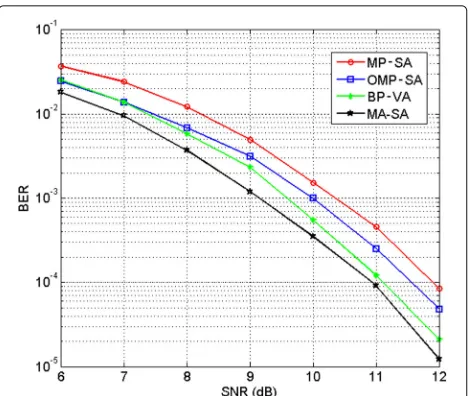
In order to further investigate the performance of the proposed method, we consider a scenario in which a short training sequence is transmitted. In this case, we compare the MA-SA with methods that combine greedy algorithms with the VA, which attains the ML solution in the presence of AWGN. We can use MP, OMP, and BP to estimate the sparse channel using the training sequence. When training is available, each channel tap value can be estimated (rather than estimating only channel sparsity). Thus, sequential detection methods such as the VA can be applied using the estimated channel. Here, we com-pare the performance of the proposed MA-SA to that of BP-VA, MP-SA, and OMP-SA. (The BP-VA approach is selected for performance comparison because the individ-ual algorithms show strong performance. SC-EM is not included in this simulation, since it uses iterative EM other than the combination of greedy algorithms and sequential detection methods using graph structure.) Simulations are constructed under the same conditions described above. A known length-10 training sequence is appended to each length-100 block of data. Performance results for the four methods are shown in Fig. 6. We observe that the pro-posed MA-SA method still achieves the best performance among the four methods due to its iterative update of the channel within the tree-search process. BP-VA outper-forms the MP/OMP-SA; by solvingl1−l2optimization problems, BP can provide a better channel estimate than the MP/OMP, and the VA is able to achieve the ML estimation of the transmitted sequence.

5.2 Efficiency comparison

Fig. 6Performance comparison between MP-SA, OMP-SA, BP-VA, and MA-SA. The performance for each method is computed using a length-10 training sequence for a 10-tap channel with three active taps

compute the metric for a given path, the MP-SA method detects the channel sparsity first and computes the met-ric using the estimated channel sparsity, while the MA-SA method computes the initial metric ford(0) =[0,. . ., 0] and updates the metric with the sparsity detection. The metric computation for MP-SA using the estimated chan-nel sparsity and the initial metric computation for MA-SA have the same complexity. Therefore, to compare the com-plexity of MP-SA and MA-SA, we need only compare their computational complexity in channel sparsity detection. This complexity depends on the estimate of the active channel length,Lˆa, which is affected by the channel itself and by the noise level.

For a path with lengthn, MP-SA constructs ann×Lh sig-nal matrixX(n). At thep-th iteration, a length-nresidual vectorbpis projected onto the direction of each column ofX(n),ai,i=1,. . .,Lh. For each iteration,Lhinner prod-uct computations are performed. Furthermore,Lhnorm computations (inner products) of ai must be performed to scale the projection as shown in [12]. Therefore, after the estimated active channel lengthLˆ(MP-SA)a is obtained,

ˆ

L(MP-SA)a iterations must be performed to estimate the sparsity. Hence, MP-SA must performLˆ(MP-SA)a Lh+Lh =

ˆ

L(MP-SA)a +1

Lh inner product computations between two length-nvectors.

For a length-n path, at each iteration, the MA-SA

computes the metric update σ0 σ1

√

θ exp

−_2θσβ2

r(yxn) T

V(:,j)V(j, :)r(yxn)

. We do not consider the

multi-Table 1Computational complexity of the MP-SA and MA-SA methods

Complexity for channel sparsity detection at each path

Inner product computations

MP-SA ˆL(MP-SA)a +1

Lh

MA-SA ˆL(MA-SA)_a +1 Lh−1₂ˆL(MA-SA)a

The computational complexity for each method is measured in terms of the number of inner product computations required for channel sparsity detection along each path of the tree

plications of the constants σ0 σ1

√

θ and

β

2θσ2, since

they are just a one-time operation. Thus, the com-plexity for each metric update is the inner product of two length-n vectors, V(j, :) and r(yxn). To obtain the final metric, the metric update is computed

ˆ

L(MA-SA)a +1 Lh−12Lˆ (MA-SA) a

times, so MA-SA must

perform Lˆ(MA-SA)a +1 Lh−12Lˆ (MA-SA) a

inner prod-uct computations between two length-n vectors. The complexity comparison between the MP-SA and MA-SA methods is summarized in Table 1.

WhenLa is known at the receiver, both methods will terminate after theLa-th loop,Lˆ(MP-SA)= ˆL(MA-SA)=La. Comparing the complexity expressions we derived above, MA-SA performs La(La+1)

2 fewer inner product computa-tions than MP-SA at each path of the tree. While La(La+1)

2 may not be a large number, the computational savings occur along each path. In the application of the SA, a large number of paths will be extended, particularly when SNR is low, making the complexity reduction achieved by MA-SA significant.

WhenLais unknown, we use numerical results to make complexity comparisons. We evaluate the complexity of the MP-SA and MA-SA methods empirically by com-paring the average number of paths extended and the total number of inner product computations for each data block. As in the earlier simulations, we consider a length L_h=10 channel withLa=3 active taps. Results from 103 simulations are averaged, and the complexity comparison for various SNR values is shown in Table 2.

The results show that MA-SA extends fewer paths than MP-SA, particularly when SNR is low, due to the robust-ness of the MA-SA method to noise in channel sparsity detection. As we can see from Table 2, for an SNR of 6 dB, MA-SA performs about 3×105fewer inner prod-uct computations than MP-SA, resulting in a roughly 75% reduction in complexity.

6 Conclusions

Table 2Computational complexity comparison between MP-SA and MA-SA

Complexity comparison

MP-SA MA-SA

Paths extended Inner product computations Paths extended Inner product computations

6 dB 17,184 945,120 8279 255,997

8 dB 9695 484,752 5183 202,137

10 dB 4748 237,904 3090 128,150

12 dB 3606 151,452 1343 45,976

The comparison is made for lengthLh=10 sparse channels withLa=3 active taps

no training sequence is used in the system and proposed a computationally efficient blind sequential detection method using the MA and SA, both tree-search-based algorithms. A Gaussian mixture model is used to describe the sparse ISI channel, and the MA is applied to blindly estimate the channel sparsity. The estimated channel spar-sity is then used to compute the path metrics within the SA, which guides the search in a tree. The MA and SA are combined to achieve blind sequential detection.

For performance comparison, we combined conven-tional sparse channel estimation techniques such as MP, OMP, and BP with the SA to jointly estimate the sparse channel and transmitted sequence; we considered both blind and semi-blind (when a short training sequence is available) cases. Simulation results show that the pro-posed MA-SA method is more likely to correctly estimate the channel sparsity along each extended path of the tree than are the comparison methods. Conventional methods are more likely to generate inaccurate channel estimates when SNR is low, which not only limits the performance of the detector but also increases the computational bur-den. Additionally, we have shown the computational effi-ciency of the MA-SA approach when the number active taps, La is known or unknown. Numerical results for unknownLashow that proposed MA-SA method achieves both significant computational savings and performance improvement when compared to conventional methods.

Future work will consider alternate channel models and simplifications to accommodate longer channels. We will also investigate the design of a modified SA-MA approach that exploits a multiple tree structure [32] to further improve the efficiency of blind sequential detection.

Acknowledgements

The authors would like to thank the editor and anonymous reviewers for their constructive comments which helped to improve the quality of this paper.

Funding

This material is based upon work supported by the National Science Foundation under Grant No. CCF-1053932 (CAREER).

Authors’ contributions

The authors declare that all authors have materially participated in the research and have contributed equally to this paper. Both authors read and approved the final manuscript.

Ethics approval and consent to participate

Not applicable

Consent for publication

Not applicable

Competing interests

The authors declare that they have no competing interests.

Publisher’s Note

Springer Nature remains neutral with regard to jurisdictional claims in published maps and institutional affiliations.

Author details

1_{Department of Bioengineering, George Mason University, 4400 University Dr.,} Fairfax, VA 22030, USA.2_{Department of Electrical and Computer Engineering,} George Mason University, 4400 University Dr., Fairfax, VA 22030, USA.

Received: 19 July 2017 Accepted: 27 December 2017

References

1. SUH Qureshi, Adaptive equalization. Proc. IEEE.73(9), 1349–1387 (1985) 2. M Chen, J Tuqan, D Zhi, A quadratic programming approach to blind

equalization and signal separation. IEEE Trans. Signal Process.57(6), 2232–2244 (2009)

3. R Liu, Y Inouye, Blind equalization of MIMO-FIR channels driven by white but higher order colored source signals. IEEE Trans. Inf. Theory.48(5), 1206–1214 (2002)

4. I Santamaria, C Pantaleon, L Vielva, J Ibanez, Blind equalization of constant modulus signals using support vector machines. IEEE Trans. Signal Process.52(6), 1773–1782 (2004)

5. V Zarzoso, P Comon, Blind and semi-blind equalization based on the constant power criterion. IEEE Trans. Signal Process.53(11), 4363–4375 (2005)

6. L Tong, G Xu, T Kailath, Blind identification and equalization based on second-order statistics: a time domain approach. IEEE Trans. Inf. Theory.

40(2), 340–349 (1994)

7. S Chen, W Yao, L Hanzo, Semi-blind adaptive spatial equalization for MIMO systems with high-order QAM signalling. IEEE Trans. Wireless Commun.7(11), 4486–4491 (2008)

8. H Nguyen, BC Levy, The expectation-maximization Viterbi algorithm for blind adaptive channel equalization. IEEE Trans. Commun.53(10), 1671–1678 (2005)

9. N Seshadri, Joint data and channel estimation using blind trellis search techniques. IEEE Trans. Commun.42(234), 1000–1011 (1994) 10. JK Nelson, AC Singer, inThe 40th IEEE Annual Conference on Information

Sciences and Systems. Bayesian ML sequence detection for ISI channels, (Princeton, 2006), pp. 693–698

11. RJ Johnson, P Schniter, TJ Endres, JD Behm, DR Brown, RA Casas, Blind equalization using the constant modulus criterion: a review. Proc. IEEE.

86(10), 1927–1950 (1998)

13. T Kang, RA Iltis, inIEEE International Conference on Acoustics, Speech and Signal Processing. Matching pursuits channel estimation for an underwater acoustic OFDM modem, (Las Vegas, 2008), pp. 5296–5299 14. Z Hussain, J Shawe-Taylor, DR Hardoon, C Dhanjal, Design and

generalization analysis of orthogonal matching pursuit algorithms. IEEE Trans. Inf. Theory.57(8), 5326–5341 (2011)

15. D Middleton, Non-Gaussian noise models in signal processing for telecommunications: new methods an results for class A and class B noise models. IEEE Trans. Inf. Theory.45(4), 1129–1149 (1999)

16. T Zhang, J Dan, G Gui, IMAC: Impulsive-mitigation adaptive sparse channel estimation based on Gaussian-mixture model. Comput Res Repository.abs/1503.00800(2015). https://arxiv.org/abs/1503.00800 17. GG Raleigh, JM Cioffi, Spatio-temporal coding for wireless

communications. IEEE Global Telecommun. Conf.3, 1809–18143 (1996) 18. IE Telatar, Capacity of multi-antenna Gaussian channels. Eur. Trans.

Telecommun.10, 585–595 (1999)

19. GJ Foschini, MJ Gans, On limits of wireless communications in a fading environment when using multiple antennas. Wirel. Pers. Commun.6, 311–335 (1998)

20. R Johannesson, K Zigangirov,Fundamentals of convolutional coding. (IEEE Press, New York, 1999)

21. RE Blahut,Algebraic codes for data transmission. (Cambridge University Press, New York, 2003)

22. JB Anderson, Limited search trellis decoding of convolutional codes. IEEE Trans. Inf. Theory.35(5), 944–955 (1989)

23. JE Gentle,Matrix algebra: theory, computations, and applications in statistics. (Springer, New York, 2007)

24. S Chen, XC Yang, L Hanzo, in6th IEE International Conference on 3G and Beyond. Blind joint maximum likelihood channel estimation and data detection for single-input multiple-output systems, (Washington, DC, 2005), pp. 1–5

25. SF Cotter, BD Rao, Sparse channel estimation via matching pursuit with application to equalization. IEEE Trans. Commun.50(3), 374–377 (2002) 26. F Xiong, A Zerik, E Shwedyk, Sequential sequence estimation for channels

with intersymbol interference of finite or infinite length. IEEE Trans. Commun.38(6), 795–804 (1990)

27. G Mileounis, N Kalouptsidis, B Babadi, V Tarokh, in17th IEEE International Conference on Digital Signal Processing (DSP). Blind identification of sparse channels and symbol detection via the EM algorithm, (Corfu, 2011), pp. 1–5

28. M Elad,Sparse and redundant representations: from theory to applications in signal and image processing. (Springer, New York, 2010)

29. CR Berger, S Z, JC Preisig, P Willett, Sparse channel estimation for multicarrier underwater acoustic communication: from subspace methods to compressed sensing. IEEE Trans. Signal Process.58(3), 1708–1721 (2010)

30. J Huang, CR Berger, S Zhou, J Huang, Comparison of basis pursuit algorithms for sparse channel estimation in underwater acoustic OFDM. IEEE OCEANS. 1–6 (2010). http://ieeexplore.ieee.org/document/5603522/ 31. W Zhou, Computationally efficient equalizer design. PhD thesis, George

Mason University (2014)