R E S E A R C H
Open Access
Numerical solution of nonlinear stochastic
Itô–Volterra integral equations based
on Haar wavelets
Jieheng Wu
1, Guo Jiang
1*and Xiaoyan Sang
1*Correspondence: [email protected] 1School of Mathematics and Statistics, Hubei Normal University, Huangshi, P.R. China
Abstract
In this paper, an efficient numerical method is presented for solving nonlinear stochastic Itô–Volterra integral equations based on Haar wavelets. By the properties of Haar wavelets and stochastic integration operational matrixes, the approximate solution of nonlinear stochastic Itô–Volterra integral equations can be found. At the same time, the error analysis is established. Finally, two numerical examples are offered to testify the validity and precision of the presented method.
Keywords: Haar wavelets; Stochastic integration operational matrixes; Stochastic Itô–Volterra integral equations
1 Introduction
Stochastic integral equations are widely applied in engineering, biology, oceanography, physical sciences, etc. There systems are dependent on a noise source, such as Gaussian white noise. As we all know, many stochastic Volterra integral equations do not have ex-act solutions, so it makes sense to find more precise approximate solutions to stochastic Volterra integral equations. There are different numerical methods to stochastic Volterra integral equations, for example, orthogonal basis methods [1–10], wash series methods [11,12], and polynomials methods [13–16].
In [1], Fakhrodin studied linear stochastic Itô–Volterra integral equations (SIVIEs) through Haar wavelets (HWs). In [3], Maleknejad et al. also considered the same in-tegral equations by applying block pulse functions (BPFs). In [9], Heydari et al. solved linear SIVIEs by the generalized hat basis functions. Meanwhile, in line with the same hat functions, Hashemi et al. also presented the numerical method of nonlinear SIVIEs driven by fractional Brownian motion [8]. Moreover, Jiang et al. applied BPFs to solve two-dimensional nonlinear SIVIEs [7]. In a general way, Zhang studied the existence and uniqueness solution to stochastic Volterra integral equations with singular kernels and constructed an Euler type approximation solution [17,18].
Inspired by the discussion above, we use HWs to solve the following nonlinear SIVIE:
x(v) =x0(v) +
v
0
k(u,v)σx(u)du+
v
0
r(u,v)ρx(u)dB(u), v∈[0, 1), (1)
wherex(v) is an unknown stochastic process defined on some probability space (Ω,F,P),
k(u,v) andr(u,v) are kernel functions foru,v∈[0, 1), andx0(v) is an initial value function.
B(u) is a Brownian motion and0vr(u,v)ρ(x(u))dB(u) is Itô integral.σandρare analytic functions that satisfy some bounded and Lipschitz conditions.
In contrast to the above papers [1,3,7–9], the differences of this paper are as follows. Firstly, we construct a preparation theorem to deal with the nonlinear analytic functions. Secondly, the error analysis is strictly proved. Finally, compared with the reference [8], the numerical solution is more accurate and the calculation is simpler because of the use of HWs. Moreover, the rationality and effectiveness of this method can be further supported by two examples.
The structure of the article is as follows.
In Sect.2, some preliminaries of BPFs and HWs are given. In Sect.3, the relationship between HWs and BPFs is shown. In Sect.4, the approximate solutions of (1) are derived. In Sect.5, the error analysis of the numerical method is demonstrated. In Sect.6, the validity and efficiency of the numerical method are verified by two examples.
2 Preliminaries
BPFs and HWs have been widely analysed by lots of scholars. For details, see references [1,3].
2.1 Block pulse functions
BPFs are denoted as
ψi(v) =
⎧ ⎨ ⎩
1 ih≤v< (i+ 1)h,
0 otherwise,
fori= 0, . . . ,m– 1,m= 2Lfor a positive integerLandh=m1,v∈[0, 1). The basic properties of BPFs are shown as follows:
(i) disjointness:
ψi(v)ψj(v) =δijψi(v), (2)
wherev∈[0, 1),i,j= 0, 1, . . . ,m– 1, andδijis Kronecker delta;
(ii) orthogonality:
T
0
ψi(v)ψj(v)dt=hδij;
(iii) completeness property: for everyg∈L2[0, 1), Parseval’s identity satisfies
1
0
g2(v)dv= lim
m→∞ m i=0
(gi)2ψi(v)
2
, (3)
where
gi=
1
h
1
0
The set of BPFs can be represented by the followingm-dimensional vector:
Ψm(v) =
ψ0(v), . . . ,ψm–1(v)
T
, v∈[0, 1). (4)
From the above description, it yields
Ψm(v)ΨmT(v) =
⎛ ⎜ ⎜ ⎜ ⎜ ⎝
ψ0(v) 0 · · · 0 0 ψ1(v) · · · 0
..
. ... . .. ... 0 0 · · · ψm–1(v)
⎞ ⎟ ⎟ ⎟ ⎟ ⎠
m×m
,
ΨmT(v)Ψm(v) = 1,
Ψm(v)ΨmT(v)Fm= DFmΨm(v),
whereFm= (f0,f1, . . . ,fm–1)Tand DFm=diag(Fm).
Furthermore, for anm×mmatrix M, it yields
ΨmT(v)MΨm(v) =MˆTΨm(v),
whereMˆ is anm-dimensional vector and its entries equal the main diagonal entries of M. In accordance with BPFs, every functionx(v) which satisfies square integrable conditions in the interval [0, 1) can be approached as follows:
x(v)xm(v) = m–1
i=0
xiψi(v) =XmTΨm(v) =ΨmT(v)Xm,
where the functionxm(v) is an approximation of the functionx(v) and
Xm= (x0,x1, . . . ,xm–1)T. (5)
Similarly, every functionk(u,v) defined on [0, 1)×[0, 1) can be written as
k(u,v) =ΨmT1(u)KΦm2(v), where K = (kij)m1×m2 with
kij
1
h1h2
1
0
1
0
k(u,v)ψi(u)φj(v)du dv, (6)
andh1=m11,h2=m12.
2.2 Haar wavelets
The notation and definition of HWs are introduced in this section (also see [1]). The set of orthogonal HWs is defined as follows:
hi(v) = 2
l
whereh0(v) = 1,v∈[0, 1), and
h(v) =
⎧ ⎨ ⎩
1 0≤v<1 2, –1 12≤v< 1.
For HWshn(v) defined in [0, 1), we have
1
0
hi(v)hj(v)dv=δij, (7)
whereδijis the Kronecker delta.
In accordance with HWs, every functionx(v) that satisfies square integrable conditions can be approached as follows:
x(v) =c0h0(v) + ∞
i=1
cihi(v), v∈[0, 1),i= 2l+z, 0≤z< 2l,l≥0,l,z∈N, (8)
where
ci=
1
0
x(v)hi(v)dv, i= 0 or i= 2l+z, 0≤z< 2l,l≥0,l,z∈N. (9)
We can see that whenm= 2L, equation (8) can be rewritten as
x(v) =c0h0(v) +
m–1
i=1
cihi(v), i= 2l+z, 0≤z< 2l,l= 0, 1, . . . ,L– 1.
Obviously, the vector form is as follows:
x(v)CTmHm(v) =HmT(v)Cm, (10)
whereHm= (h0(v),h1(v), . . . ,hm–1(v))T andCm= (c0,c1, . . . ,cm–1)Tare HWs and Haar co-efficients, respectively.
Similarly, every functionk(u,v) defined on [0, 1)×[0, 1) can be approached as follows:
k(u,v) =HmT(u)KHm(v),
where K = (kij)m×mwith
kij=
1
0
1
0
k(u,v)hi(u)hj(v)du dv, i,j= 0, 1, . . . ,m– 1.
3 Haar wavelets and BPFs
Some lemmas about HWs and BPFs are introduced in this section. For a detailed descrip-tion, see the reference [1].
Lemma 3.1 Suppose that Hm(v)andΨm(v)are respectively given in(10)and(4),Hm(v)
can be written in accordance with BPFs as follows:
whereQ= (Qij)m×mand
Qij= 2
j
2h
i–1
2j– 1 2m
, i,j= 1, 2, . . . ,m,i– 1 = 2l+z, 0≤z< 2l.
Proof See [1].
Lemma 3.2 Suppose thatQis given in(11),then we have
QTQ=mI,
whereIis an m×m identity matrix.
Proof See [1].
Lemma 3.3 Suppose that F is an m-dimensional vector,we have
Hm(v)HmT(v)F=F˜Hm(v),
whereF˜is an m×m matrix andF˜= QFQ¯ –1,F¯=diag(QTF).
Proof See [1].
Lemma 3.4 Suppose thatMis an m×m matrix,we have
HmT(v)MHm(v) =MHˆ m(v),
whereMˆ =NTQ–1is an m-dimensional vector and the entries of the vector N are the
diag-onal entries of matrixQTMQ.
Proof See [1].
Lemma 3.5 Suppose thatΨm(v)is given in(4),we have
v
0
Ψm(u)duPΨm(v),
where
P=h 2
⎛ ⎜ ⎜ ⎜ ⎜ ⎜ ⎜ ⎜ ⎝
1 2 2 · · · 2 0 1 2 · · · 2 0 0 1 · · · 2
..
. ... ... . .. ... 0 0 0 · · · 1
⎞ ⎟ ⎟ ⎟ ⎟ ⎟ ⎟ ⎟ ⎠
m×m
.
Lemma 3.6 Suppose thatΨm(v)is given in(4),we have Firstly, a useful result for HWs is proved.
Proof According to the disjointness property of HWs, we can deduce
σxm(v)
= aj
xm(v)
j
= aj
c0h0(v) +c1h1(v) +· · ·+cm–1hm–1(v)
j
= aj
cj0,cj1, . . . ,cjm–1Hm(v)
=σT(Cm)Hm(v),
thus,
σxm(v)
=σT(Cm)Hm(v) =HmT(v)σ(Cm). (12)
Similarly,
ρxm(v)
=ρT(Cm)Hm(v) =HmT(v)ρ(Cm). (13)
The proof is completed.
Now, in order to solve (1), we approximatex(v),x0(v),k(u,v), andr(u,v) in following forms by HWs:
x(v)xm(v) =CmTHm(v) =HmT(v)Cm, (14)
x0(v)x0m(v) =C0
T
mHm(v) =HmT(v)C0m, (15)
k(u,v)km(u,v) =HmT(u)KHm(v) =HmT(v)KTHm(u), (16)
r(u,v)rm(u,v) =HmT(u)RHm(v) =HmT(v)RTHm(u), (17)
whereCm andC0m are HWs coefficient vectors, K and R are HWs coefficient matrices.
Substituting approximations (12)–(17) into (1), we have
CmTHm(v) =C0TmHm(v) +HmT(v)KT
v
0
Hm(u)HT(u)σ(Cm)du
+HmT(v)RT
v
0
Hm(u)HmT(u)ρ(Cm)dB(u).
By Lemma3.3, we get
CmTHm(v) =C0TmHm(v) +HmT(v)KT
v
0 ˜
σ(Cm)Hm(u)du
+HmT(v)RT
v
0 ˜
ρ(Cm)Hm(u)dB(u).
Applying Lemmas3.7and3.8, we get
then by Lemma3.4, we derive
CmTH(v) =C0TmH(v) +AˆT0H(v) +BˆT0H(v), (18)
where A0= KTσ(C˜m)Λand B0= RTρ(C˜m)ΛB.
For nonlinear equation (18), a series of methods, such as simple trapezoid method, Simpson method, and Romberg method, are often introduced in the numerical analysis courses. In this paper, the function of fsolve in MATLAB is used to solve equation (18).
5 Error analysis
In contrast to the articles [1,3], we will give a strict and accurate error analysis in this section. Firstly, we recall two useful lemmas.
Lemma 5.1 Suppose that function x(u), u∈[0, 1)satisfies the bounded condition and e(u) =x(u) –xm(u),where xm(u)is m approximations of HWs of x(u),then
e2L2([0,1))=
1
0
e2(u)du≤Oh2. (19)
Proof See [1].
Lemma 5.2 Suppose that the function x(u,v)satisfying the bounded condition is defined onD= [0, 1)×[0, 1)and e(u,v) =x(u,v) –xm(u,v),where xm(u,v)is m approximations of
HWs of x(u,v),then
e2L2(D)=
1
0
1
0
e2(u,v)du dv≤Oh2. (20)
Proof See [1].
Secondly, lete(v) =x(v) –xm(v), wherexm(v),x0m(v),km(u,v), andrm(u,v) arem
approx-imations of Haar wavelets ofx(v),x0(v),k(u,v), andr(u,v), respectively.
e(v) =x(v) –xm(v)
=x0(v) –x0m(v)
+
v
0
k(u,v)σx(u)–km(u,v)σ
xm(u)
du
+
v
0
r(u,v)ρx(u)–rm(u,v)ρ
xm(u)
dB(u). (21)
Lastly, the main convergence theorem is proved.
Theorem 5.1 Suppose that analytic functionsσandρsatisfy the following conditions:
(i) |σ(x) –σ(y)| ≤l1|x–y|,|ρ(x) –ρ(y)| ≤l3|x–y|; (ii) |σ(x)| ≤l2,|ρ(y)| ≤l4;
where x,y∈R,constant li> 0,i= 1, 2, . . . , 6.Then
Proof For (21), we have
Eem(v)2
or
By Gronwall’s inequality, it follows that
By using (19) and (20), we have
Ii≤wih2, i= 1, 2, . . . , 6.
So we can get
T
0
Eem(v)
2
dv≤3w1+ 6l22w2+ 6l42w3
+αeαT3w4+ 6l22w5+ 6l42w6
h2
≤Oh2,
where constantwi> 0,i= 1, 2, . . . , 6.
The proof is completed.
6 Numerical examples
In this section, some examples are given to verify the validity and rationality of the above method.
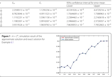
Table 1 Whenm= 24, error meansEm, error standard deviationsEs, and confidence intervals are given in this table
v Em Es 95% confidence interval for error mean
Lower Upper
1
16 2.1422688×10
–5 1.0711344×10⁻⁶ 8.4307964×10⁻⁸ 4.2416924×10⁻⁶ 2
16 6.9693462×10
–5 3.4846731×10⁻⁶ 1.7016633×10⁻⁷ 1.3799305×10⁻⁵ 3
16 6.0556726×10⁻⁵ 3.0278363×10⁻⁶ 1.4766843×10⁻⁷ 1.1990231×10⁻⁵ 4
16 5.9652419×10⁻⁵ 2.9826209×10⁻⁷ 2.1384868×10⁻⁷ 1.1811179×10⁻⁵ 5
16 2.9736896×10⁻⁵ 1.4868448×10⁻⁶ 6.69011884×10⁻⁸ 5.8879054×10⁻⁶
Table 2 Whenm= 25, error meansEm, error standard deviationsEs, and confidence intervals are given in this table
v Em Es 95% confidence interval for error mean
Lower Upper
1
32 2.2590513×10⁻⁶ 1.1295256×10⁻⁶ 4.5181026×10⁻⁸ 4.4729216×10⁻⁶ 2
32 8.7823046×10⁻⁶ 4.3911523×10⁻⁶ 1.7564609×10⁻⁷ 1.7388963×10⁻⁵ 3
32 1.1192231×10⁻⁵ 5.5961158×10⁻⁶ 2.2384463×10⁻⁷ 2.2160618×10⁻⁵ 4
32 1.1983301×10
–5 5.9916507×10⁻⁶ 2.3966603×10⁻⁷ 2.3726937×10⁻⁵ 5
32 3.9319526×10
–5 1.9659763×10⁻⁵ 7.8639053×10⁻⁷ 7.7852663×10⁻⁶
Figure 1 m= 24, simulation result of the
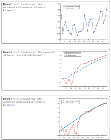
Figure 2 m= 25, simulation result of the approximate solution and exact solution for Example6.1
Figure 3 m= 24, simulation result of the approximate
solution and mean solution for Example6.2
Figure 4 m= 25, simulation result of the
approximate solution and mean solution for Example6.2
Example6.1 Consider the nonlinear SIVIE [6,8]
x(v) =x0(v) –a2
v
0
x(u)1 –x2(u)du+a
v
0
1 –x2(u)dB(u), v∈[0, 1),
where
x(v) =tanhaB(v) + arctanh(x0)
.
In this example,a= 301 andx0(v) = 101. The error meansEm, error standard deviations
Es, and confidence intervals of Example6.1form= 24 andm= 25are shown in Table1
and Table2, respectively. The error meansEmand error standard deviationsEsare
ob-tained by 104trajectories. Compared with Table 2 in [8],E
interval is smaller under the same confidence level. Moreover, the comparison of exact and approximate solutions of Example6.1form= 24andm= 25is displayed in Fig.1and Fig.2, respectively.
Example6.2 Consider the nonlinear SIVIE [17,18]
x(v) = 1 +
v
0
e–(v–u)sinx(u)du+
v
0
e–(v–u)cosx(u)dB(u), v∈[0, 1).
The mean and approximate solutions of Example6.2form= 24andm= 25are respec-tively given in Fig.3and Fig.4, where the mean solution is obtained by 104trajectories.
Funding
This article is funded by NSF Grants 11471105 of China and Innovation Team of the Educational Department of Hubei Province T201412. These supports are greatly appreciated.
Availability of data and materials
No availability of data and material.
Competing interests
The authors declare that they have no competing interests.
Authors’ contributions
The authors have made the same contribution. All authors read and approved the final manuscript.
Publisher’s Note
Springer Nature remains neutral with regard to jurisdictional claims in published maps and institutional affiliations.
Received: 4 June 2019 Accepted: 2 December 2019 References
1. Mohammadi, F.: Numerical solution of stochastic Itô–Voltterra integral equations using Haar wavelets. Numer. Math., Theory Methods Appl.9, 416–431 (2016)
2. Reihani, M.H., Abadi, Z.: Rationalized Haar functions method for solving Fredholm and Volterra integral equations. J. Comput. Appl. Math.200, 12–20 (2007)
3. Maleknejad, K., Khodabin, M., Rostami, M.: Numerical solution of stochastic Volterra integral equation by a stochastic operational matrix based on block pulse function. Math. Comput. Model.55, 791–800 (2012)
4. Maleknejad, K., Basirat, B., Hashemizadeh, E.: Hybrid Legendre polynomials and block-pulse functions approach for nonlinear Volterra–Fredholm integro-differential equations. Comput. Math. Appl.61, 2821–2828 (2011) 5. Maleknejad, K., Khodabin, M., Rostami, M.: A numerical method for solving m-dimensional stochastic Itô–Volterra
integral equations by stochastic operational matrix. Comput. Math. Appl.63, 133–143 (2012)
6. Ezzati, R., Khodabin, M., Sadati, Z.: Numerical implementation of stochastic operational matrix driven by a fractional Brownian motion for solving a stochastic differential equation. Abstr. Appl. Anal.2014, Article ID 523163 (2014) 7. Jiang, G., Sang, X.Y., Wu, J.H., Li, B.W.: Numerical solution of two-dimensional nonlinear stochastic Itô–Volterra integral
equations by applying block pulse function. Adv. Pure Math.9, 53–66 (2019)
8. Hashemi, B., Khodabin, M., Maleknejad, K.: Numerical solution based on hat functions for solving nonlinear stochastic Itô–Volterra integral equations driven by fractional Brownian motion. Mediterr. J. Math.14, 1–15 (2017)
9. Heydari, M.H., Hooshmandasl, M.R., Ghaini, F.M.M., Cattani, C.: A computational method for solving stochastic Itô–Volterra integral equations based on stochastic operational matrix for generalized hat basis functions. Mediterr. J. Math.270, 402–415 (2014)
10. Mirzaee, F., Hadadiyan, E.: Numerical solution of Volterra–Fredholm integral equations via modification of hat functions. Appl. Math. Comput.280, 110–123 (2016)
11. Balakumar, V., Murugesan, K.: Single-term Walsh series method for systems of linear Volterra integral equations of the second kind. Appl. Math. Comput.228, 371–376 (2014)
12. Blyth, W.F., May, R.L., Widyaningsih, P.: Volterra integral equations solved in Fredholm form using Walsh functions. ANZIAM J.45, 269–282 (2003)
13. Mohamed, D.S., Taher, R.A.: Comparison of Chebyshev and Legendre polynomials methods for solving two dimensional Volterra–Fredholm integral equations. J. Egypt. Math. Soc.25, 302–307 (2017)
14. Maleknejad, K., Sohrabi, S., Rostami, Y.: Numerical solution of nonlinear Volterra integral equations of the second kind by using Chebyshev polynomials. Appl. Math. Comput.188, 123–128 (2007)
15. Ezzati, R., Najafalizadeh, S.: Application of Chebyshev polynomials for solving nonlinear Volterra–Fredholm integral equations system and convergence analysis. Indian J. Sci. Technol.5, 2060–2064 (2012)
17. Zhang, X.C.: Euler schemes and large deviations for stochastic Volterra equations with singular kernels. J. Differ. Equ.
244, 2226–2250 (2008)
18. Zhang, X.C.: Stochastic Volterra equations in Banach spaces and stochastic partial differential equation. J. Funct. Anal.