Volume 2008, Article ID 732145,13pages doi:10.1155/2008/732145
Research Article
Energy Efficiency Comparison of MIMO-Based
and Multihop Sensor Networks
George Bravos and Athanasios G. Kanatas
Wireless Communications Laboratory, Department of Technology Education and Digital Systems, University of Piraeus, 80 Karaoli and Dimitriou Street, 18534 Piraeus, Greece
Correspondence should be addressed to George Bravos,[email protected]
Received 11 July 2007; Revised 16 October 2007; Accepted 12 December 2007
Recommended by Richard Kozick
Wireless sensor networks (WSNs) demand the implementation of energy-aware techniques and low-complexity protocols in all layers. Recently, a MIMO-based structure has been proposed to offer enhanced energy savings in WSNs. In this paper, we examine and compare MIMO-based WSN with a multihop transmission in terms of energy efficiency. The results depend on the network density, the channel conditions, and the distance to the destination node. We reach analytical expressions to calculate threshold values of these parameters, which determine the areas where the MIMO-based structure outperforms multihop transmission. Moreover, we present a detailed analysis of the dissipated power during a sensor node s operation, to prove that as microelectronics develops, the MIMO-based architecture will outperform the equivalent multihop structure for most of the cases examined. Finally, we implement a simple cooperative node selection algorithm to achieve higher energy gains in the MIMO approach, and we examine how this algorithm affects the calculated thresholds.
Copyright © 2008 G. Bravos and A. G. Kanatas. This is an open access article distributed under the Creative Commons Attribution License, which permits unrestricted use, distribution, and reproduction in any medium, provided the original work is properly cited.
1. INTRODUCTION
One of the most important characteristics of a WSN is that the sensor nodes usually operate on small batteries, which are difficult to replace, and thus have restricted sources of energy [1]. Consequently, the design of such networks should focus primarily on improving the performance in terms of energy efficiency.
A technique that has been recently introduced in WSNs focusing on energy efficiency is cooperative networking. A sensor network may be seen as a multi-input/multioutput (MIMO) system, where a sensor node is assigned the role of a transmitting or receiving antenna of the MIMO structure. This structure may offer enhanced energy gains for a WSN, depending on the distance between the Tx and Rx sides of the system.In [2], it was proved that a MIMO system supports higher data rates without increasing transmission power, which is equivalent to the conclusion that MIMO systems demand less transmission energy than single-input/single-output (SISO) systems for the same throughput require-ments. This view was used in [3], where the authors proved that under certain conditions a sensor network may operate
based on a MIMO structure. Moreover, there is a critical dis-tance between the transmitter and the receiver above which MIMO transmission is more energy-efficient than SISO. This topic was furtherly discussed in [4], where a thorough study towards the energy efficiency of MIMO-based schemes was carried out.
A very interesting extension of the work on MIMO-based WSNs is an architecture called MIMO-sensor net-works with mobile agents (M-SEMNA), proposed in [5]. According to M-SEMNA, several neighboring nodes are se-lected to transmit information cooperatively, whereas the data sink is equipped with multiple antennas. Such receiver though does not suffer from energy limitations; thus the re-sults obtained, however promising they are, are not applica-ble to several WSN applications. In [6], the proposed proto-col is based on extending the traditional low-energy adaptive clustering hierarchy protocol (LEACH) by incorporating the cooperative MIMO communication.
nodes that form the virtual antenna array in order to trans-mit the data seriously affects the network’s energy consump-tion. In [7], a new MAC protocol based on cooperation is proposed. No specific relay algorithm is defined though. An interesting scheme is proposed in [8] including two diff er-ent policies for selecting the best relay node, based mainly on channel estimates. Finally, an algorithm that considers also the remaining energy of the neighbor nodes before choosing the cooperation node may be found in [6].
Although several comparisons regarding energy con-sumption have been made between MIMO-based and sim-ple SISO-based networks, no comparison has been made—to our knowledge—versus the energy consumed by a network based on multihop transmission. One of the contributions of this paper is the investigation of the parameters that af-fect the energy efficiency of a MIMO-based sensor network in comparison to a SISO multihop-based network. In partic-ular, we focus on the distance between the transmitter and the receiver, the node density, and the channel conditions. Moreover, we estimate the threshold values over which the MIMO structure is more energy-efficient. Two cases of mul-tihop networks are investigated regarding the transmission range of the nodes. On the first one, a typical range value is used, while on the second one an optimization algorithm is applied.
Considering the rapid technology evolution, we elaborate on the results using three different examined scenarios re-garding the electronics used in the hardware and the power they dissipate. In addition, we implement a simple but very effective cooperative node selection algorithm, and estimate its effect on the threshold values of the examined parame-ters. For both cases, we prove that as technology develops, the thresholds that determine MIMO structure’s energy effi -ciency become looser, and in the short future MIMO trans-missions should be applied in WSNs for most cases.
The remainder of the paper is organized as follows.
Section 2presents a brief description of the MIMO and mul-tihop structures on sensor networks, along with the mod-els used for energy consumption and distances between nodes in the network. The energy estimation analysis is done in Section 3, followed by threshold values estimations and future tendencies that are gathered and marked upon in
Section 4.Section 5describes the cooperation node selection algorithm and its effect on the estimated thresholds. Finally, a summary is made inSection 6, along with some useful con-clusions.
2. SISO AND MIMO MULTIHOP APPROACH: MODELING ENERGY AND SPACE
2.1. SISO and MIMO-based transmission
The most common communication way in WSNs is to for-ward the data through multiple hops, using intermediate nodes that are deployed between the source and the destina-tion. LetHmultidenote the total number of hops needed for
the data to reach the destination node, and letEbbe the
en-ergy consumed for transmitting one bit of data at each hop.
Transmitter side Mtnodes
Long-haul transmission
Receiver side Mrnodes
Destination node
Local transmissions
Figure1: MIMO-based approach for WSNs.
Then, the total energy consumption for transmittingLbits of data from a source to a destination node is given by
Emultihop=HmultiLEb. (1)
On the other hand, the basic idea in the MIMO-based structure for WSNs is that there areMtneighbor nodes with
data to be transmitted to a destination node. Each node broadcasts its information to all neighbor nodes using diff er-ent time slots (local transmissions), and in what follows, the transmission sequence is encoded according, for example, to the Alamouti diversity codes [2]. Theith node then transmits the sequence that theith antenna would transmit in an Alam-outi MIMO system (long-haul transmission). On the receiver side, theMr nodes, with the destination node included,
re-ceive the encoded data, and theMr−1 nodes forward the data
to the destination node after quantizing each symbol intonr
bits. The MIMO approach is explained in [3] and summa-rized inFigure 1.
The energy required to complete a transmission ofLbits based on this MIMO structure is given by [3]
EMIMO
=LMIMO Mt
i=1
Etb,i+LMIMOElbMt+
LMIMOMt
b
Mr−1
j=1 Er
b,jnr,
(2)
whereEt
b, Erb, Elbare the energy consumptions for
transmit-ting and receiving one bit of data in the transmitter side and the receiver side and for the long-haul transmission, respec-tively, andLMIMO=L/Mt.In general,Ebis a function of the
path loss factornand the average range of the nodesd. In the case of local transmissions, the range depends on the distance between two neighbouring nodes,dk.For long-haul
trans-missions, we use the average distance between source and destination nodes, denoted by D. We assume that channel conditions are approximately the same at both the receiver side and the transmitter side; so the value of the path loss fac-tornis the same for all cases. Finally, (LMIMOMt)/bexpresses
Table1: Typical values of energy model parameters.
a 1.33
Psyn 25 mW
Pc 22.9 mW
Ttr 5μs
Pdetector 5 mW
2.2. Energy model
The energy (Eb) consumed to transmit and receive one bit is
expressed by
Eb=
Pt+aPt+Pc+Pdetector
Ton+ 2PsynTtr
L . (3)
In (3),aexpresses the energy consumption in the power am-plifier and depends on the modulation used [9,10], Ttr is
the transition time needed for the node to change from the “sleep” to the “awake” mode, andPsyn, Pdetector, Pcrepresent
the power dissipated in the frequency synthesizers, the de-tector, and the rest of the circuitry.Ton is the time needed
for the transmission ofLbits, depending on the transmis-sion rate Rb(Ton = L/Rb), andPt is the transmitted power
calculated by the link budget equation [11]
Pt(d,n)(dBW)
=PL(d,n)(dB)+
Eb,required
N0(dB)+Rb(dBHz)−204(dBW/Hz)+S(dB),
(4)
wherePLis the average path loss accounting for large-scale fading,Sis a safety margin,−204 dBW/Hz is a typical value ofN0, andEb,required/N0depends on the channel, the
modu-lation used, and the target BER [12]. The average path loss is calculated by a single slope model. Typical values for the parameters used in the energy model are shown inTable 1. More details on the complete energy model used to estimate Ebcan be found in [9].
2.3. Space model
Assume that M sensor nodes are randomly deployed in a square surface with length 2R on each edge. Using a two-dimensional Poisson distribution model [13], the distance between two neighboring nodes, defined asdk, is a random
variable (r.v.) with a mean value that is expressed with the help of node densityρsas [13]
Edk
=dk=
1 4ρs =
R √
M,
ρs= M
4R2.
(5)
During the sensor network’s operation, a node called
source nodesenses a piece of data and has to deliver it to the
destination node, which may be any of theM nodes of the network. The distance betweensource nodeanddestination
Source node
d
dk
dnNext hopx
D
Destination node
Figure2: Space modeling.
node, denoted byD, is also an r.v. that according to [13,14], has a mean value given by
E[D]=D= R
3 √
2 + ln1 +√2. (6)
The last variable that has to be modeled is the distance between thesource nodeand thenext hop, which is used in the case of multihop transmission and is denoted bydn. The next hopis in the direction of the destination node, and it is selected to be the closest node to the rangedof thesource. In order to modeldn, we model the distancexbetween the
range limits (d) and thenext hop. Hence,
dn=d−x. (7)
Using the two-dimensional Poisson model, we estimate the mean value ofxby
E[x]=x 1
4ρs+ 1/R2
πd. (8)
Details on the derivation of (8) may be found in
Appendix A. The distance model is summarized and de-picted inFigure 2.
3. ENERGY CONSUMPTION ANALYSIS
According to the framework and definitions given in
Section 2, the energy consumption in the cases of MIMO-based and multihop-MIMO-based structures may be furtherly ana-lyzed as follows.
3.1. Energy consumption of MIMO-based network
Using the energy and space models presented inSection 2
and assuming thatEt
b =Erb =Eb(dk,n) andEbl =Eb(D,n),
we derive
EMIMO
=LMIMOMtEb(d,n)
1 +
Mr−1
nr
Using (3) forEb(d,n) andEb(D,n), we evaluate the energy
consumed for the transmission ofLbits of data for a MIMO-based network according to
EMIMO
whereRb,local, Rb,long-haul are the data rates (in bits per
sec-ond) used in the local and the long-haul transmissions, re-spectively, estimated according to [3], and the factorsEf,iare
given by
j=local, long-haul,
Ef,4=
whereTon,local, Ton,long-haulrepresent the time needed for the
transmission ofLbits according to the data rate. The vari-abled, that expresses the average transmission range of the nodes, depends ondkand thereforeρs. From (10), it is
obvi-ous that the main factors affecting energy consumption are the path loss factor, the distanceDbetweensourceand desti-nation nodes, and the network’s densityρs.
It should be clarified that in the long-haul transmis-sions, the average range is equal toD, which means that the Mt transmitting nodes are able to adjust their transmission
power to achieve that specific average range. That is feasible if we assume that thedestination nodebroadcasts a pilot sym-bol during the initial phase of the network’s operation, using a globally known transmission power levelPt,dest. Each node
can estimate the transmission power needed to reach the des-tinationnode using the knowledge of the path loss, which is derived by comparing the power level of the received signal, Pr,dest, to the transmission power level, as shown in the
fol-lowing equation:
PL=Pt,dest−Pr,dest. (12)
It is also possible that the node with the role of the desti-nationchanges periodically. In that case, every time a destina-tionnode change happens, a pilot symbol has to be sent again from the newdestinationto notify the nodes of the network. Finally, considering local transmissions in MIMO structure, they are done assuming that each node is able to exchange data with its neighbor nodes (dn=dk).
3.2. Energy consumption of SISO multihop approach
When the network is based on the traditional multihop ap-proach, then the total energy needed for the transmission of Lbits is given by (1). The average number of hops,Hmulti, for
a given distance Dis
Hmulti
Using this expression along with the energy model de-scribed by (3), we get the form of (14), describing the energy consumption during SISO multihop transmission:
Emultihop=LEb(d,n)Hmulti
Once again, the energy consumption depends on three main factors: the path loss factorn, the distanceD, and the network density ρs, expressed via the distance dk. The
to-tal performance of such a multihop structure is straightfor-wardly dependant on the transmission power,Pt, and
there-fore the transmission ranged. Hence, we will examine two different cases considering the value of d in the multihop operation. According to the first case, dis the range needed for the first neighbor node to be thenext hop.Hence,dn=dk,
and dis given by (7) that reduces to
d=dk+x. (15)
Alternatively, we utilize an optimization algorithm that esti-mates the value of Pt and henced, and minimizes the
to-tal energy consumption on multihop-based networks, as it is expressed by (14). Minimizing that expression, forn=2, we get
and dnis estimated by (7). The transmission power used is
defined according to
For values ofn >2, the expressions ofdoptare more
com-plicated and are computed numerically. More details regard-ing the optimization of the transmission power and average range for minimizing total energy consumption in multihop networks are given in [10]. We should mention that for very small values ofD, the multihop optimization algorithm may result in worse performance than that of simple multihop ap-proach. That is because these values of Dactually refer to cases where the destination node is within the range of the source node, and thus only a single hop is needed for the data to be delivered.
Having estimated (10) and (14), the problem is defined as follows. Calculate the threshold values for the parameters n,ρs,Dfor which
0 0.1 0.2 0.3 0.4 0.5 0.6 0.7 0.8
Energ
y
consump
ti
on
(joule)
0 20 40 60 80 100
DistanceD(meters) SISO, total
MIMO, total MIMO,Etrans
MIMO,Ecirc
SISO,Etrans
SISO,Ecirc
Figure3: Energy consumption segregation for SISO and MIMO
architectures versus distance.
Table2: Indicative parameters value.
Bits to be transmitted (L) 10000
Frequency (f) 2500 (MHz)
nr 10
Mt 2
Mr 2
Target bit error rate (BER) 10−5
Antenna gains (Gt×Gr) 5 dBi
S 10 dB
Reference distance (d0) 0.5 m
R 50 m
3.3. Power dissipation analysis
Before proceeding with the analysis of (18), we focus on distinguishing the energy consumed by the circuitry of the node, denoted withEcirc, from the energy that depends on
the transmission power,Etrans, based on the model presented
inSection 2:
Eb=Etrans+Ecirc,
Etrans=
(a+ 1)PtTon
L ,
Ecirc=
Pc+Pdetector
Ton+ 2PsynTtr
L .
(19)
The importance of the power dissipated in the circuitry on the total performance of the MIMO architecture is obvi-ous fromFigure 3, which depicts the total energy consump-tion for MIMO 2×2 and SISO architectures versus the dis-tance of the long-haul transmission, based on the parameters shown in Tables1and2and explained in detail in [9]. Dis-tance in local transmissions is assumed to be fixed and equal
Table3: Examined scenarios.
Scenario 1 Ecirc=10 uJ
Scenario 2 Ecirc=1 uJ
Scenario 3 Ecirc=0.1 uJ
to 1m, while the constellation sizes used are derived from the rate-optimization algorithms presented in [10]. According to that figure, a 2×2 MIMO structure is more energy-efficient than a SISO-based WSN when the distance between the re-ceiver and the transmitter sides is greater than 20 m. We may observe though that the term that actually increases the en-ergy consumption in the MIMO approach isEcirc, which
in-cludes the energy consumed by all electronics that do not have to do with transmission power, such as filters, mixers, and so on. If we consider the rapid deployment in microelec-tronics during the last years, then it is highly expected that more energy-efficient circuitry will be available soon. There-fore, MIMO structure is expected to become more energy-efficient. This is not the case with the SISO approach though, whereEtransinserts the greater parts of energy consumption.
Less energy consumed in the circuitry results in lower dis-tance thresholds and thus makes the MIMO structure more energy-efficient for almost any case.
In order to examine the effect of Ecirc on the distance
thresholds above which the MIMO structure is more energy-efficient than SISO multihop transmission, we use three dif-ferent scenarios for the value ofEcircas shown inTable 3.
Sce-nario 1 corresponds to the values ofTable 1. As shown in the next section, reducing Ecirc results in remarkable changes
regarding the threshold values that determine when MIMO-based structures are more energy-efficient.
4. THRESHOLDS ESTIMATION AND TENDENCIES
4.1. System analysis
In this section, we proceed with the estimation of the thresh-old values for the three crucial factors affecting the energy consumption, namely, the path loss factorn, the distanceD, and the network densityρs. Indeed, we calculate the
thresh-old values for which (18) is satisfied. We examine the per-formance of three different transmission structures. The first two are based on forwarding the data using Hmultimultiple
nodes, while in the next section a selection algorithm is pro-posed. For all examined schemes, we use a target BER value equal to 10−5, while in the MAC layer we assume a simple
slotted Aloha protocol. As far as the way the data is routed within the network to reach the destination node, we use an assumption commonly found in the literature, according to which information about the destination node is included into the data packets. For the figures that presented this point forward, the following configuration is assumed. Regarding the energy model, the values shown inTable 1are used, while typical values for all other variables considering the evalua-tion of energy consumpevalua-tion are summarized inTable 2. For both local and long-haul transmissions, we assume Rayleigh fading channels. As far as the density is concerned, we con-sider a fixed deployment area with R=50 m, while the total number of nodes,M, varies. According to the value ofM, we get the node density from (5), measured in nodes per surface A(nodes/A). In our case,Ais an area of 1 m2, and the
den-sity may take values from 0.003 to 0.05, and thus the average distance between neighbor nodes varies between 2.2 and 9 m.
4.2. Interference issues
In wireless networks, and especially in networks with the characteristics of WSNs, a very important issue to be taken into consideration is interference. According to [15], the to-tal interference at a node mand time kis given by
Im[k]= NP
l=1
Ptγlm[k] + D
j=1
Ptγjm[k], (20)
assuming that the interference at each relay can be due to either other sources transmitting simultaneously or due to the other intermediate nodes which are in their transmission phase at time k and have started reception at timek−1. In (20), γi jis the channel gain between nodesi,j,D is the
total number of interfering relays, and NPis the number of
sources at timek.
In our case though, where only two nodes cooperate to transmit data using the Alamouti coding, (20) includes one single factor as only one node transmits simultaneously with our source node. Hence, interference as expressed in (20) is limited. It is well understood [16] that the number of inter-ferers clearly increases the interference problem in wireless networks. The fact that in our scenarios we only focus on cases where one interference node is present reduces the im-pact of such a problem.
Moreover, basic channel state knowledge, which is present in our scenarios, significantly affects the network’s tolerance in interference [17]. In the same paper [17], the authors prove that the better the channel conditions are, the more tolerant the MIMO structures in interference will be.In particular, it is shown that unless the channel condi-tions are severe (e.g.,n =3.5), the effect of interference on MIMO structures’ performance is negligible. As we analyt-ically discuss in the next subsections, MIMO-based WSNs outperform multihop transmission schemes mainly in sce-narios where the channel conditions are good. Hence, we may conclude that in such scenarios, which are of the main
10−1
100
Energ
y
consump
ti
on
(joule)
0 20 40 60 80 100
DistanceD(m) MIMO,n=2
Multihop opt,n=2
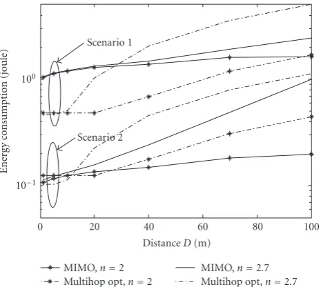
MIMO,n=2.7 Multihop opt,n=2.7 Scenario 1
Scenario 2
Figure4: Total energy consumption versusDwhenρs=0.01 (M=
100) andn=2.0,n=2.7.
interest in this paper, interference can be assumed as negligi-ble.
Finally, it has been stated in [18] that Alamouti-based transmission provides a very good performance in interfer-ence reduction. Hinterfer-ence, we focus on scenarios that use this specific simple space-time coding scheme, in order not to in-crease complexity as well as the interference effect.
4.3. Solving subject to the distanceD
Solving inequality (18) for the distance betweensourceand
destination nodes,we get the polynomial expression
Ef,3 long-haul L(α+ 1) Rb,long-haul
Dn
−
Ef,4+Ef,3 localdn
(α+ 1)/Rb,local
dn
D
+
Ef,1+Ef,2Ef,3 localdk nα+ 1
Rb,local
>0,
(21)
wheredn and d may take values according to two diff
er-ent cases, simple and optimized, as already explained in
Section 3.2. A numerical solution algorithm for the polyno-mial is presented inAppendix B. In what follows, results will be presented based on the general form described by (21).
10−2
numerical solution of (21) (Dthreshold,numerically ≈ 24.21 m).
Using (6), we derive that D = 38.25 m, and therefore the MIMO structure is expected to perform better than the sim-ple multihop case for scenario 2. In the case of n = 2.7, we may reach a similar conclusion, as if scenario 2 is used instead of scenario 1, the threshold value above which the MIMO scheme outperforms optimized multihop transmis-sion reduces from 30 to 10 m.
4.4. Solving subject to the path loss factorn
Inequality (18) leads us to the form of (22), when trying to solve it with respect to the path loss factorn:
Inequality (22) is n-grade exponential, and may be solved numerically according to the method described in
Appendix C. The case of a network consisting of 100 nodes with D =40 m is depicted inFigure 5. Although through-out the paper we mainly examine cases of 2< n <3, in this first figure we expand the path loss factor’s range to 4, in or-der to examine the performance for worse channel condi-tions. Regarding the 2nd scenario, for example, the thresh-old value below which the MIMO structure becomes more energy-efficient isn <2.8. This value may also be verified nu-merically (nthreshold,numerically ≈2.77). Similar threshold
val-ues may be extracted for the other two scenarios. Obviously,
10−1
Figure6: Total energy consumption versusnandDwhenρs=0.01
(M=100).
when the channel becomes much worse (e.g.,n >3), the en-ergy consumption of the MIMO-based structure increases significantly. That is mainly due to the long-haul transmis-sion, where the effect of the large values of n is greater. Hence, regarding the examined structures, energy gains may be feasible by MIMO schemes mainly for path loss factor val-ues up to 3, as the threshold valval-ues mainly appear for the cases of 2< n <3.
A more thorough view of the interrelation between the values of path loss factor and the distance between source
anddestination nodesis shown inFigure 6. We examine the case of a network consisting of 100 nodes, and the compar-ison is made between the MIMO and the optimized multi-hop scenarios for the 2nd scenario. We therefore conclude that multihop structure is more energy-efficient for the cases where Dand nare both large, for example, n > 2.7 and D > 50. There is also a small area where multihop outper-forms MIMO if D <10 andn <2.4.
4.5. Solving subject to network densityρs
The last variable examined regarding the effect on energy ef-ficiency of MIMO-based sensor networks is the node density ρs. Density is expressed through the average distance between
two neighbor nodes,dk, and inequality (18) takes a form that
depends on the multihop scenario examined. If the transmis-sion range is set according to (15), then the inequality to be solved is the polynomial
0
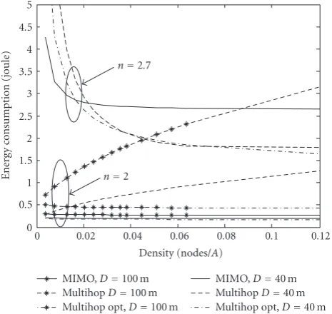
Figure7: Total energy consumption versus density whenn=2 and D=40,D=100.
This equation may as well be solved numerically using the method described inAppendix B. When the optimization al-gorithm is used and transmission range is set according to (16), then we get the form of inequality (24) derived for the
Having clarified the effect of potential reduction ofEcirc
on the MIMO structure’s performance, in this paragraph we restrict our investigation to scenario 2 and we focus on the interrelation betweenD,n, andρs. The energy consumption
for the three examined schemes is depicted inFigure 7for the cases of n=2 or 2.7 andD=40 m,D=100 m. Let us first examine the case ofn = 2. As one observes forD = 40 m, increasing the density mainly affects the first case of mul-tihop structure. MIMO structure, on the other hand, per-forms slightly worse than optimized multihop for all densi-ties. If we increase the distance Dto 100 m, the MIMO-based network is less affected, and hence it becomes more energy-efficient than both multihop schemes. The simple multihop structure is still highly affected by the density, and its per-formance gets worse as the density increases. This was antic-ipated since in this case the next hop is the closest node in the network, and therefore increasing the density increases the number of hops. On the other hand, when the optimized
−100
Figure8: Energy gains inserted forD=40 m and different network densities.
distance is used, the energy consumption slightly decreases with the increase of the density up to a point beyond which the dominant factor in (16) is no more the distance dkbut
rather the rest terms that are fixed.
Increasing the path loss factor to 2.7 though significantly changes the interrelation between density and energy con-sumption. Now, the performance of all schemes in terms of energy efficiency improves as the density increases. The im-provement is more rapid in the multihop schemes, and thus there is an upper threshold in the density below which the MIMO-based network is more energy-efficient.
Figure 8gives an overview of the gains inserted due to MIMO structure with respect to the simple multihop case, for several network densities, and forD=40 m. In general, when the channel is good, the MIMO-based scheme offers remarkable gains in terms of total energy consumption. The gains become greater as the network density increases. On the other hand, whenn >2.5, sparser networks offer greater gains for the MIMO case. Depending on the density, there is a critical value of nabove which the multihop scheme be-comes more energy-efficient.
4.6. Performance regarding time delay
Apart from energy efficiency, a critical issue regarding the performance in WSNs is the time delays inserted until the data arrives at the destination node. Hence, it is important to investigate the effect of the MIMO-based structure on the time delay with respect to simple multihop transmission.
Assuming that the data is transmitted using multiple hops,then the time needed for the data to be delivered to the destination node is
where tlocalis the time needed for the data to be transmitted
from one node to the next hop node.
On the other hand, for 2×2 MIMO-based structures, the time delay may be expressed as follows:
TMIMO=2tlong-haul+tadd, (26)
where tlong-haul,tadd are the time delays for the long-haul
transmission and for the additional symbols that are needed to be exchanged for the formation of the virtual MIMO transceivers, respectively. Using the Alamouti coding scheme, 2 long-haul time slots are needed for the data to be delivered. The data rates used in local and long-haul transmissions are the same; so we assume that
tlocal=tlong-haul=Ton, (27)
whereTon, as defined earlier, is the time needed for the packet
of data to be transmitted from one node to another. More-over, regardingtadd, it includes the time spent for the pilot
symbols needed to form the virtual MIMO transceiver as well as the time needed for the actual data to be exchanged, both at the transmitter’s side and the receiver’s side. At the transmitter’s side, the essential transmission is the one be-tween the first node that senses the data and the node cho-sen for cooperation. At the receiver’s side, data has to be cho-sent to the destination node from the node chosen for cooper-ation. Therefore, 2Ton is required for actual data
transmis-sions. Having the cooperation node chosen randomly among neighbors and using only 2×2 systems, we conclude that one pilot symbol is enough for the transceiver’s formation and the time delay inserted is negligible. Hence,
tadd=2Ton. (28)
Combining the above, we may derive
Tmultihop=HmultiTon,
TMIMO4Ton.
(29)
According to the scenarios examined in this paper, we de-rive from (13) that Hmultimay vary from 4 up to 18.
There-fore, we may conclude that using 2×2 MIMO-based struc-tures does not insert any additional time delays.
However, assume thattaddtakes greater values than 2Ton.
It is clear from (29) that depending on the value ofHmulti, TMIMO may be still less than Tmultihop for values of taddup
to 8Ton. Of course there are some cases where MIMO-based
structure may insert greater time delays than multihop sce-narios, but this requires thattaddbe significantly higher than
estimated.
5. THRESHOLD ESTIMATION AND COOPERATIVE NODE SELECTION ALGORITHM
In this section, we implement a simple cooperative node se-lection algorithm in the 2×2 MIMO structure, to achieve enhanced energy efficiency. The algorithm’s implementation affects the threshold values estimated in this section. We will investigate these effects and re-examine the interrelations be-tween the critical variables already mentioned.
5.1. The cooperative node selection algorithm
We implement a simple cooperative node selection algo-rithm based on estimations of the channel conditions in the links between neighboring nodes. This algorithm applies to MIMO structures described in previous sections. We intro-duce a novel metric TEL (total energy lifetime), that is de-fined as follows.
Assume that the channel in both local and long-haul transmissions suffers from log-normal shadowing and that each node has to choose among Nneighbor nodes for co-operation. That is, the received power at each node j (j =
1, 2,. . .,N) after a source node transmits a packet of datais estimated by
Prj=Pt−PL
dj
+Gt+Gr
=Pt−PL
dj
−χ+Gt+Gr,
(30)
where Gt,Gr are the gains of the transmitter and receiver
antennas, respectively, and henceforth they are set to 0 dBi. All factors are expressed in logarithmic scale. Shadowing is expressed by the normally distributed variableχ, with zero mean and variance equal to 5 dB. If we assume that at the be-ginning of the network’s operation each node sends a pilot symbol and waits for acknowledgments to specify its neigh-bors, then the knowledge of the transmission power level combined with the knowledge of the acknowledgement’s power level allows the node to be aware of the path loss given by (30). As the path loss values experienced by the links greatly affect the total energy consumed in the network, TEL is a function ofPL(dj): TELj=f
PLdj
.
Apart from the total energy consumed in the network, another important metric to measure energy efficiency is life-time. When energy is uniformly consumed within the net-work, increased lifetime is assured. Therefore, TEL also in-cludes information about the energy left at each node j, de-noted withEleftj : TELj= f(Eleftj ).
The cooperation node (CN) is selected according to
TELj= PLdj
Eleftj
,
CN=arg minTELj
.
(31)
The CN selection is made by the source node as well as the destination node, at the transmitter and receiver sides, re-spectively. In our case, only 2×2 systems are examined, and hence both source and destination nodes will choose only one node to cooperate with. Since the selection is based on both the channel state and the energy left at each neighbor, the optimum CN is re-estimated every time a node has data to retransmit. Upon selection, the CNs at the trans-mitter and receiver sides are informed by the source or the destination node, respectively.
5.2. Effect of CN selection on general performance
10−2
10−1
100
101
102
103
Energ
y
consump
ti
on
(joule)
0 20 40 60 80 100
DistanceD(m) MIMO,n=2.5
MIMO with CN selection,n=2.5 MIMO,n=3
MIMO with CN selection,n=3
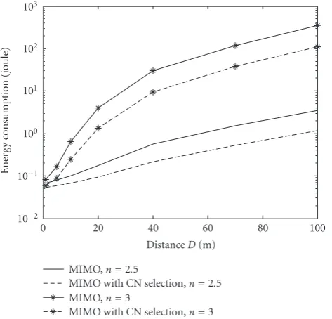
Figure 9: Effect of CN algorithm on total energy consumption,
M=100.
performance of a MIMO-based WSN using the proposed scheme. The implementation of the specific algorithm in our networks requires the transmission of some additional pilot messages. The fact that we consider only 2×2 systems re-sults in the additional energy consumption being much less than the energy needed for the actual data transmission. Nev-ertheless, that energy cost has been taken into account in the following. InFigure 9, we observe the total energy con-sumption in a network consisting of 100 nodes for two dif-ferent cases regarding the path loss factor. It is obvious that the gains inserted due to CN selection become remarkably greater as the channel conditions get worse. For the case of n=2.5, energy gains are close to 100% for a distance equal to 25 m.
As already stated, the implemented CN algorithm also focuses on increasing the network’s lifetime by distributing uniformly the energy consumption within the network. This is also depicted inFigure 10, for a network consisting of 100 nodes andn =2.5. Here, lifetime is defined as the number of packets delivered until the first node runs out of energy. The algorithm’s effect on the lifetime depends on the number of possible neighbors Nfrom which the source node has to choose the CN, as more neighbors result in more uniformly distributed energy consumption. Hence, we examine three different cases regardingN. One observes that even when the choice is made out of two nodes, gains are inserted in terms of lifetime. As the number of neighbor nodes increases, the gains become greater. The decreased lifetime observed when fewer nodes are used in the transmitter’s side is due to the fact that fewer nodes are used to transmit the same amount of data, and hence they remain out of energy faster.
The implementation of such an algorithm may also affect the time delays until the data is delivered to the destination node. Both the source and the destination nodes now search among all their neighbors in order to find the best one to
101
102
103
104
Lifetime
(n
umber
o
f
p
ac
ke
ts)
0 20 40 60 80 100
DistanceD(m) CN selection
No CN selection
N=2 N=4
N=9
Figure10: Effect of CN algorithm on network’s lifetime;n=2.5, M=100.
cooperate with. On the other hand, the actual data will be transmitted only once between cooperation nodes, just as in the simple case described inSection 4.6, after the CN selec-tion has been made. Hence, the addiselec-tional time delays are due to the time needed for the completion of the CN selec-tion (tCN selection), which includes only pilot symbols:
tadd=2Ton+tCN selection. (32)
The value of tCN selection depends on the number of pilot
symbols needed for the cooperation node to be chosen, and consequently on the number of neighbors of both the source and destination nodes. Having in mind though that the time needed for a pilot symbol is much less than the delays in-serted by sending the actual data and knowing that in general the MIMO-based structure inserts less time delays than the multihop transmission based on (29), we conclude that the CN selection algorithm does not affect the system’s perfor-mance in terms of total time delays.
5.3. Effect of CN selection on threshold values
Figure 11summarizes the node selection algorithm effect on the threshold values Dfor the case of n = 2.7. When the node density is small (ρs=0.003), the MIMO-based network
seems to operate more energy-efficiently than the multihop-based network for any value of D > 31 m. This threshold value drops to 25 m, when the CN selection algorithm is used. Increasing network’s density decreases the threshold values of Dthat determine the critical points for the MIMO structure, but the improvement inserted due to CN selection remains remarkable.
0 1 2 3 4 5 6
Energ
y
co
nsumption
(joule)
0 20 40 60 80 100
DistanceD(m) Multihop opt
MIMO MIMO with CN
ρs=0.003
ρs=0.05
Figure11: Effect of node selection algorithm on thresholds
esti-mations whenn = 2.7 and (ρs = 0.003) (M =30), (ρs = 0.05)
(M=500).
10−1
100
101
102
Energ
y
co
nsumption
(joule)
2
2.5
3
Path
loss factor 0
50
100
D(m)
Multihop opt MIMO with CN
Figure12: Total energy consumption when CN selection is used
versusnandDwhenρs=0.0127 (M=100).
structure now outperforms the optimized multihop scheme for almost any examined case regarding path loss factor and distanceD.
Finally,Figure 13provides the total energy gains inserted when MIMO structure is used in combination with CN se-lection, with reference to the case of multihop transmission. The depicted results are for D = 40 m and show that the energy gains are remarkable for most of the combinations of the network density and the path loss factor. Moreover, we compare the gains with the ones provided by the simple MIMO case inFigure 8, and we observe that, especially for
−80
−60
−40
−20 0 20 40 60 80 100
Energ
y
gains,
M
IMO
o
ve
r
m
ultihop
(%)
2 2.2 2.4 2.6 2.8 3
Path loss factor ρs=0.003
ρs=0.01
ρs=0.021
ρs=0.03
ρs=0.05
Figure13: Energy gains inserted with CN selection forD=40 m
and different network densities.
2.2< n <2.8 and for low densities, the additional gains in-serted are greater than 20%.
6. CONCLUSIONS
APPENDICES
A. ESTIMATINGE[x]
If dis the range of the node, then the probability of having a node in an area betweend−xandd+x, wherex∈(0,dk),
Then, the probability of no node being in the same area is given by
and the relative c.d.f. is therefore
c.d.f.=1−P(X > x)=1−
From the c.d.f., we may straightforwardly compute the p.d.f. as
The mean value of the variablexis then estimated as follows:
E[x]=x= dk
0 PDF·x dx= −dkA
M+B1−AM+1,
(A.5)
where the factors A,Bare given by
A=R2−πddk
and thus all factors except B are equal to zero. Then, the above expression reduces to
E[x]≈ 1
B. NUMERICAL SOLUTIONS FOR POLYNOMIALS
Thenth-grade polynomials, that appear in the cases of solv-ing them versus Danddk, should be converted to
integer-grade polynomials. Assuming that n takes discrete values in [2.0 3.0] with step equal to 0.1, we use the substitutions y1=D1/10, y2=dk
Finally, we estimate itscompanion matricesCm1,Cm2as
Cm1=
The solutions of the polynomials may then be estimated by calculating the eigenvalues ofCm1,Cm2, from whichDand dkmay be easily extracted.
C. SOLVING THE EXPONENTIAL EQUATION
In order to solve the exponential equation, we will first turn it into a polynomial one, and then use the method described inAppendix B. The problem to be solved is described by
where
a=
Ef,3 long-haul L
(α+ 1) Rb,long-haul
,
b=
Ef,3 local((α+ 1)/Rb,local)D dn
,
c=
Ef,2Ef,3 localα+ 1 Rb,local
,
d=
Ef,1 Ef,4D
dn
,
A=D, B=d, C=dk.
(C.2)
We use the following transformation set:
X=An, Y=Bn, Z=Cn (C.3)
from which, using logarithms, we get
X=YK, K=lnA
lnB,
Z=YL, L=lnC
lnB.
(C.4)
Equations (C.3) and (C.1) lead to
aX−bY+cZ+d=0 (C.5)
which, with the help of (C.4), results in the polynomial
aYK−bY+cYL+d=0. (C.6)
Equation (C.6) may then be solved using the method de-scribed inAppendix B.
ACKNOWLEDGMENT
This work has been done within the framework of the project PENED 2003 entitled “Data transmission techniques in Wireless Sensor Networks”, partially funded by the Euro-pean Union.
REFERENCES
[1] I. F. Akyildiz, W. Su, Y. Sankarasubramaniam, and E. Cayirci, “A survey on sensor networks,” IEEE Communications Mag-azine , vol. 40, no. 8, pp. 102–114, 2002.
[2] G. J. Foschini and M. J. Gans, “On limits of wireless commu-nications in a fading environment when using multiple anten-nas,” Wireless Personal Communications , vol. 6, no. 3, pp. 311–335, 1998.
[3] S. Cui, A. J. Goldsmith, and A. Bahai, “Energy-efficiency of MIMO and cooperative MIMO techniques in sensor net-works,” IEEE Journal on Selected Areas in Communications , vol. 22, no. 6, pp. 1089–1098, 2004.
[4] S. K. Jayaweera, “Energy analysis of MIMO techniques in wire-less sensor networks,” inProceedings of the 38th Annual Confer-ence on Information SciConfer-ences and Systems (CISS ’04), Princeton, NJ, USA, March 2004.
[5] L. Xiao and M. Xiao, “A new energy-efficient MIMO-sensor network architecture M-SENMA,” inProceedings of the 60th IEEE Vehicular Technology Conference (VTC ’04), vol. 4, pp. 2941–2945, Los Angeles, Calif, USA, September 2004. [6] Y. Yuan, Z. He, and M. Chen, “Virtual MIMO-based
cross-layer design for wireless sensor networks,” IEEE Transactions on Vehicular Technology , vol. 55, no. 3, pp. 856–864, 2006. [7] R. Lin and A. P. Petropulu, “A new wireless network medium
access protocol based on cooperation,” IEEE Transactions on Signal Processing , vol. 53, no. 12, pp. 4675–4684, 2005. [8] A. Bletsas, A. Khisti, D. P. Reed, and A. Lippman, “A simple
co-operative diversity method based on network path selection,” IEEE Journal on Selected Areas in Communications , vol. 24, no. 3, pp. 659–672, 2006.
[9] G. Bravos and A. G. Kanatas, “Energy consumption and trade-offs on wireless sensor networks,” inProceedings of the 16th IEEE International Symposium on Personal, Indoor and Mobile Radio Communications (PIMRC ’05), vol. 2, pp. 1279–1283, Berlin, Germany, September 2005.
[10] S. Cui, A. J. Goldsmith, and A. Bahai, “Energy-constrained modulation optimization,” IEEE Transactions on Wireless Communications , vol. 4, no. 5, pp. 2349–2360, 2005. [11] B. Sklar, Digital Communications: Fundamentals and
Ap-plications , Prentice-Hall PTR, Upper Saddle River, NJ, USA, 2nd edition, 2001.
[12] M. K. Simon and M.-S. Alouini, Digital Communication over Fading Channels: A Unified Approach to Performance Analy-sis , Wiley-Interscience, New York, NY, USA, 2000.
[13] O. K. Tonguz and G. Ferrari, Ad Hoc Wireless Networks: A Communication-Theoretic Perspective , John Wiley & Sons, New York, NY, USA, 1st edition, 2006.
[14] S. Panichpapiboon, G. Ferrari, and O. K. Tonguz, “Sensor net-works with random versus uniform topology: MAC and inter-ference considerations,” inProceedings of the 59th IEEE Vehic-ular Technology Conference (VTC ’04), vol. 4, pp. 2111–2115, Milan, Italy, May 2004.
[15] S. Vakil and B. Liang, “Balancing cooperation and interference in wireless sensor networks,” inProceedings of the 3rd Annual IEEE Communications Society on Sensor and Ad Hoc Commu-nications and Networks (SECON ’06), vol. 1, pp. 198–206, Re-ston, Va, USA, September 2006.
[16] K. Jain, J. Padhye, V. N. Padmanabhan, and L. Qiu, “Impact of interference on multi-hop wireless network performance,” inProceedings of the 9th Annual International Conference on Mobile Computing and Networking (MobiCom ’03), pp. 66–80, San Diego, Calif, USA, September 2003.
[17] A. M. Abbosh and D. Thiel, “Performance of MIMO-based wireless sensor networks with cochannel interference,” in Pro-ceedings of the 2nd International Conference on Intelligent Sen-sors, Sensor Networks and Information Processing Conference (ISSNIP ’05), pp. 115–119, Melbourne, Australia, December 2005.