A dimension separation based two dimensional correlation interferometer algorithm

Ting Cheng

, Xintao Gui and Xin Zhang

Abstract

A two-dimensional correlation interferometer algorithm based on dimension separation is proposed for wideband direction finding. The original two-dimensional angle searching is divided into 2 one-dimensional searching processes in the proposed algorithm. Therefore, the computational complexity is reduced. Meanwhile the introduced interpolation process ensures the direction finding precision. Simulation results demonstrate that compared with conventional correlation interferometer algorithm, the proposed one can offer higher direction finding speed.

Keywords:Correlation interferometer, Dimension separation, Correlation coefficient, Similarity function

1. Introduction

The information contained in the received signal of an array is commonly used to determine the incoming direc-tion of an incident wave [1]. Such a configuradirec-tion is usually called as the direction finding system. In existing direction finding systems, interferometer has the advantages of high direction finding precision, simple algorithm, and high speed, therefore, it is widely applied in military and civil fields [2,3].

Phase interferometer calculates the incoming direction with measured space phase differences between receiving elements [4]. The correlation interferometer [5,6] is the most popular one among phase interferometers. It can re-duce the effect from mutual coupling and system error through comparison between measured phase difference vector and phase difference vectors in sample database [7,8]. For two-dimensional direction finding [9], the sample database consists of phase difference vectors. Each of them corresponds to a different azimuth and elevation angle pair. The number of phase difference vectors is the size of sample database, which determines the computational complexity of direction finding algorithm [10]. In order to obtain a preferable direction finding result, the size of sam-ple database should be large enough. Therefore, the involved computational complexity grows. To the best of the authors’ knowledge, the correlation interferometer

algorithm based on space angle [11] is the only algorithm that dedicates to reduce the computational complexity of conventional algorithm. Although the computational com-plexity is reduced through introducing of two space angles, the side-effect brought to direction finding precision is not investigated.

In modern direction finding environment, there are generally more than one incoming signals. In this case, wideband direction finding system based on multi-channel structure is often adopted [12], where correl-ation interferometer algorithm is used to estimate the incoming direction of signal in each channel [13]. It can be seen that as the channel number grows, the involved computational complexity will increase. The real-time measuring of direction can hardly be guaranteed. To solve the problem mentioned above, a two-dimensional correlation interferometer algorithm based on new idea of dimension separation is proposed. Two different simi-larity functions are chosen to search for azimuth angle and elevation angle, respectively, in this algorithm. Therefore, the original two-dimensional searching is divided into 2 one-dimensional searching processes. Simulation results demonstrate the effectiveness of the proposed algorithm.

2. Problem formulation

For wideband direction finding system, the frequency range of incoming signal becomes much wider. In order to capture all possible signals, the direction finding * Correspondence:citrus@uestc.edu.cn

School of Electronic Engineering, University of Electronic Science and Technology of China, Chengdu, Sichuan 611731, P. R. China

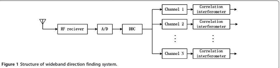
system based on multi-channel structure is always adop-ted. Figure 1 shows the system structure. In Figure 1, the received signal is digitalized with an A/D convertor, and then down converted with a DDC. The output of DDC is channelized into N channels. Because the in-coming signal may appear in each channel, direction finding should be performed on each channel. The dir-ection finding complexity will grow as the channel number N increases. Therefore, in order to guarantee the real-time of direction finding, it is advisable to de-crease the complexity of correlation interferometer. Es-pecially, in the two-dimensional direction finding case, where both azimuth and elevation angles should be estimated.

In two-dimensional direction finding, circular array is a commonly used array manifold. Consider anM -elem-ent uniformly spaced circular array (UCA) as shown in Figure 2, where R is the radius. The incident wave arrives with direction of (φ, θ), where φ is the azimuth angle and θ is the elevation angle. Consider the origin as the reference point, the received signal of element _m can be expressed as

rmð Þ ¼t Acosðω0tϕmþϕÞ ð1Þ

where A is the amplitude, ω0 = 2πf0 and f0 is the fre-quency of incoming signal, the corresponding wave-length isλ =c/f0. crepresents the light speed. ϕmis the

phase of elementmrelative to the reference point which can be expressed as

φm ¼ 2πR

λ sinθcos φ 2π

Mm

ð2Þ

According to Figure 1, after frequency mixing in RF receiver, A/D sampling and digital down-conversion, the output of DDC can be expressed as

xmð Þ ¼n Aej½ðω0ω1ÞnTsþϕϕm ð3Þ

whereTsis the sampling interval after DDC,ω1is a angle frequency that determined jointly by local oscillators in RF receiver and DDC. AssumeΔ= (ω0−ω1)Ts= 2πμ/D, then:

xmð Þ ¼n Aej½Δnþϕϕm ð4Þ

whereDis the decimator factor. When it is input into the multi-channel structure, it is filtered with a channelized fil-ter bank. The output of channelkis

ymkð Þ ¼i xmð Þen jωknh nð Þ

n¼iD ð5Þ

whereh(n) is the original low-pass filter of channelized fil-ter bank with order P, ωk = 2πk/D. According to (4), we have

ymkð Þ ¼i Aej½ϕþΔiDφm

XP1

p¼0

h pð ÞejðΔωkÞp ð₆Þ

Onceymk(i) andymk(i) are obtained, we can extract the phase difference between elements _m and _n(≠_m) accor-ding to the following operation

ymkð Þyi

nkð Þ ¼i A2jHðΔωkÞj2ej½ϕnϕm ð7Þ

where H(ω) is the frequency response of original

low-pass filterh(n). The phase difference is

Figure 1Structure of wideband direction finding system.

Figure 2Array and signal model.

ϕm;n¼ϕnϕm

¼4π_λRsin πðnmÞ

M

sinθsin φπðnþmÞ

M

problem thus is how to determine the unique direction of incident wave according to several measured phase differences precisely.

3. Conventional two-dimensional correlation interferometer

The phase differences between different elements can form a phase difference vector. Correlation interferometer determines the incoming direction of signal through the comparison of measured phase difference vector and the vectors in sample database. Assume the interested azimuth range is [φmin,φmax] and the interested elevation range is [θmin,θmax]. Divide the azimuth range withΔφand the ele-vation range with Δθ, which results in P azimuth angle values andQelevation angle values._P×Qelevation and azi-muth pair can be formed. The phase difference vectors corresponding to each angle pair formulate the sample data-base. Obviously, the size of sample database is_P×Q.

Denote the measured phase difference vector as

e

Φ∈RN1 and theith phase difference vector in database asΦ(i)∈RN×1, whereNis the element number in phase difference vector. The correlation process aims to find the phase vector that most similar with the measured vector in the sample database. The angle pair of the most similar vector is considered as the estimated in-coming direction. The process can be expressed as

argmax

wheref(·) is a function that used to measure the similar-ity between measured phase difference vector and the one in database, which is called as similarity function. Solving (9) is exactly a two-dimensional searching process. It can be seen that in order to get the azimuth and elevation angles, a similarity function that is sensi-tive both to azimuth and elevation angles should be chosen. A cosine similarity function is proposed in [14]. It has an advantage of solving phase ambiguity. According to the cosine similarity function, the similar-ity between measured vector and sample i in the data-base is calculated as

f1ð Þ ¼i

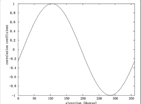
different elevation angles. If correlation coefficient f2(·) is adopted as the similarity function between measured phase difference vector and sample vector, then

f2ðφ;θ1Þð Þ ¼i transposition operation. According to (8), it can be concluded that

Substitute (13) into (12), we have

f2ðφ;θ2Þð Þ ¼i

Consider the common elevation range of (0°, 90°], we havesinθ2_sinθ1>0 and

f2ðφ;θ1Þð Þ ¼i f

φ;θ2

ð Þ

2 ð Þi ð15Þ

any information about the elevation. This phenomenon initiates the correlation interferometer based on dimen-sion separation.

4.1 Correlation interferometer based on dimension separation

Since correlation coefficient is only relevant to azimuth angle, the conventional two-dimensional searching pro-cess can be separated. In the database, the phase differ-ence vectors corresponding to a same elevation angle are chosen, measured phase difference vector is correlated to these sample vectors. The azimuth angle corresponding to the sample vector that maximizes the correlation coeffi-cient can be considered as the estimated azimuth angle. Once the estimated azimuth angle is obtained, the phase

difference vectors corresponding to the estimated azimuth angle are chosen. The measured phase difference vector is compared with these sample vectors where the similarity function chosen in this step should be sensitive to the ele-vation angle. f1(·) in (10) is chosen here. The elevation angle corresponding to the sample vector that has the lar-gest similarity is the estimated elevation angle. Obvi-ously, conventional two-dimensional searching process is divided into 2 one-dimensional searching processes in this way.

In order to increase the direction finding precision, a two-dimensional interpolation [15] is introduced after 2 one-dimensional searching processes. RememberP and

Q are the number of discrete azimuth and elevation

defined in Section Conventional two-dimensional correl-ation interferometer. Assume the index of estimated azi-muth angle is _pamong the sequence {1, 2, . . ., _P}, and the index of estimated elevation angle is_q among the se-quence {1, 2, . . .,Q}. In the sample database, the angle pairs that contiguous to the estimated angle pair are the

ones with index of (_p − 1, _q + 1), (_p, _q + 1),

(_p + 1, _q + 1), (_p − 1, _q), (_p + 1, _q), (_p − 1, _q − 1), (_p, _q − 1), and (_p + 1, _q − 1). Combining with the estimated angle pair, a small sample database with nine sample vectors can be formulated as shown in Figure 5, where the similarities between measured phase differ-ence vector and the vectors in small sample database are denoted as _si,_i = 0, 1, . . ., 8. They are calculated with_f1 (·). Switch (_p,_q) to the origin, the index coordinates turn to be the ones in Figure 6. Perform the fitting of qua-dric surface _y = _a0 + a1x + a2y + a3xy + a4x2 + a5y2 with these nine points, the coefficients are calculated as follows

Figure 3Correlation coefficient of measured phase difference vector with sample vector.

The coordinates of surface peak are

Therefore, the azimuth and elevation angles can finally be estimated as

^

θ¼^θ0þx0:Δθ;^φ¼^φ0þy0:Δφ ð18Þ

where ^θ0 and φ^0 are the estimated azimuth and eleva-tion angles, respectively, after 2 one-dimensional sear-ching processes.

Based on above illustration, the two-dimensional cor-relation interferometer algorithm based on dimension

separation can be obtained. The steps are shown as below.

Step 1: Choose an arbitrary fixed elevation angle, and select all of the phase difference vectors corresponding to this elevation angle but different azimuth angles in sample database. Step 2: Compute the correlation coefficient between

measured phase difference vector and all chosen phase difference vectors in Step 1.

Step 3: Choose the azimuth angle corresponding to the phase difference vector which has the

maximum correlation coefficient as estimated azimuth angle and denote it asφ^₀.

Step 4: Choose all phase difference vectors which share the same azimuth angle that estimated in Step 3.

Step 5: Compute the similarity between the measured phase difference vector and all chosen phase difference vectors in Step 4 according to (10). Step 6: Choose the elevation angle corresponding to

the phase difference vector which has the maximum similarity value as estimated elevation angle and denote it as^θ0.

Step 7: Process the two-dimensional interpolation and obtain the final estimated azimuth and elevation angles according to (16)–(18).

Figure 7 shows the flow chart of above algorithm. The azimuth angle is estimated in Steps 1 to 3, where an ar-bitrary elevation angle is selected because the correlation coefficient is independent of it as shown in Figure 3. The following steps aim to estimate the elevation, where

Figure 5Diagram of small sample database.

the cosine similarity function is used for its sensitivity to the elevation angle. It is worth mentioning that if Δφ and Δθ from the database are small enough, running from Steps 1 to 6 is enough to yield a satisfactory result. Therefore, the interpolation process can be avoided. If original sample database contains P ×Qsample vectors, there are_P× Qtimes operations that are used to compute the similarities in conventional correlation interferometer algorithm. In the correlation interferometer algorithm based on dimension separation, the involved similarity

operation reduces to_P+Qtimes. The direction finding ef-ficiency thus increases.

4.2 Condition for correlation interferometer algorithm based on dimension separation

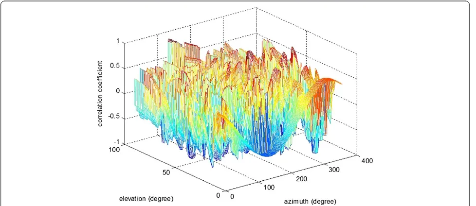
According to the steps of correlation interferometer algo-rithm based on dimension separation, the key of it is the correlation coefficient which is independent on elevation angle. Therefore, the sample vectors corresponding to any elevation angle can be used for searching to give the elem-entary estimated azimuth angle. However, this searching process is only valid in the case of no phase ambiguity, which is also the condition for the proposed algorithm. The surface of correlation coefficient in Figure 3 will change if there is phase ambiguity. Figure 8 shows an ex-ample of correlation coefficient in the existence of phase ambiguity. The dimension separation cannot be carried out for the surface which is no longer smooth.

The condition for correlation interferometer based on dimension separation will be analyzed in the following. It is actually the condition for no phase ambiguity. The model in Section Problem Formulation ignores the effect of noise. Considering the additive noise in practical situ-ation, the measured phase difference can be written as

e

ϕm;n¼ϕm;nþδm;n ¼4π_λRsin πðnmÞ

M

sinθsin φπðnþmÞ

M

þδm;n

ð19Þ

whereδm,ncan be modeled as a Gaussian random variable with zero mean and variance ofσm2,n. Assumeθ∈[θL,θH]

Figure 7Flow chart of dimension separation based correlation interferometer algorithm.

π

Substitute (21) into (20), we finally have

1α≤F πum;n

dz. For the high signal-to

-noise ratio (SNR) case, σm2,n ≪ π2, (22) can be

Substitute the form ofum,ninto (23), we finally have

R

Therefore, in order to use the correlation interferom-eter algorithm based on dimension separation, the radius to wavelength ratio must satisfy (24). For example, when α= 0.01, M = 9,R= 0.5, θL = 0°,θH= 90°, the highest

frequency that ensures no ambiguity between

contiguous element is depicted in Figure 9 according to (24). Meanwhile, the simulated result averaged among 5,000 Monte Carlo tests is also given, where the investigated phase difference is between elements 1 and 2. It can be seen that the theoretical and simulated curves match well. According to Figure 9, when SNR is 10 dB, dimension separation is valid for signals with fre-quency lower than 405 MHz. Formula (24) offers the guidance of using correlation interferometer algorithm based on dimension separation in practice.

5. Simulations

In this section, the dimension separation-based correlation interferometer algorithm is compared with conventional one in terms of direction finding precision and efficiency. In order to compare them in the same condition, (10) is used as the similarity function when two-dimensional searching or a searching that sensitive to elevation is involved in both algorithms.Itisworthmentioningthatthechangeofthisfunc-tion will not influence the comparison results. There are to-tally three kinds of algorithms to be compared hereinafter. They are conventional correlation interferometer algo-rithm, dimension separation-based correlation interferom-eter algorithm without interpolation and dimension separation-based correlation interferometer algorithm with interpolation. For simplicity of description, they are named as Algorithm 1 (conventional correlation interferometer al-gorithm), Algorithm 2 (dimension separation-based correl-ation interferometer algorithm without interpolcorrel-ation), and Algorithm 3 (dimension separation-based correlation inter-ferometer algorithm with interpolation).

5.1 Comparison of direction finding precision

Consider a 7-element UCA with a radius ofR= 1 m. Inci-dental wave arrives at the array with azimuth angle of 103°

Figure 9Highest frequency for no phase ambiguity.

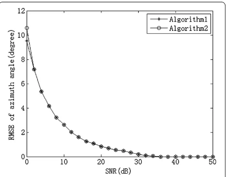
and elevation angle of 42°, and the carrier frequency is 70 MHz. Assume the interested azimuth and elevation ranges are [0°, 359°] and [0°, 90°], respectively, and the sample database is obtained with Δφ = Δθ = 1°. The following results are averaged over 2,000 Monte Carlo runs. Per-formance of algorithms is evaluated with the root mean square error (RMSE). The average time is enough to rep-resent the statistic characteristics of direction finding re-sult. AsΔφandΔθare small, interpolation is not needed. The direction finding precisions of Algorithms 1 and 2 are compared. As mentioned before, the similarity function of (10) is used in Algorithm 1. In Algorithm 2, the correl-ation coefficient similarity function (11) is used first to realize dimension separation and the similarity function of (10) is used afterwards. The RMSEs of azimuth angle esti-mate and elevation angle estiesti-mate are shown in Figures 10 and 11. It can be seen that the precision of Algorithm 2 is

consistent with that of Algorithm 1. Although the com-plexity of Algorithm 2 is reduced compared with Algo-rithm 1, they offer similar direction finding precision.

In order to investigate the effect of interpolation, assume the interested azimuth and elevation ranges remain un-changed and the sample database is obtained withΔφ= Δθ= 5°. Algorithms 2 and 3 are compared. The RMSEs of azimuth angle estimate and elevation angle estimate are shown in Figures 12 and 13. The RMSEs of azimuth and elevation estimates decrease as SNR increases. As the range of azimuth and elevation is dispersed with 5° and the real incoming angle is (103°, 42°), the RMSEs converge to 2° in Algorithm 1. However, with interpolation the RMSEs of azimuth and elevation estimates remain de-crease until SNR reaches 45 dB and converge to a much smaller degree. It can be seen that with interpolation the proposed algorithm can offer higher direction finding pre-cision. The main reason is thatΔφandΔθactually deter-mines the minimum direction finding error for a given incoming direction. The interpolation process can break through the minimum error. Therefore, ifΔφandΔθare small, the corresponding direction finding precision is sat-isfactory. Algorithm 2 can be adopted. Otherwise, Algo-rithm 3 is a better choice.

5.2 Comparison of direction finding efficiency

In order to investigate the speed up of dimension separ-ation, the direction finding efficiency of Algorithm 1 and the one based on dimension separation are compared. In

Figure 13RMSE comparison of Algorithms 2 and 3 (elevation angle).

Table 1ϕ∈[0°, 359°],θ∈[0°, 90°] with dispersion 1°

Algorithm Algorithm 1 Algorithm 2

Time (ms) 22.19240 0.12269

Speed up ratio 180.88 –

Figure 12RMSE comparison of Algorithms 2 and 3 (azimuth angle).

language to investigate the average time over 10,000 runs. Table 1 compares the direction finding efficiency when the interested azimuth and elevation ranges are [0°, 359°] and [0°, 90°], respectively, and the sample database is obtained withΔφ=Δθ= 1°. It can be seen that Algorithm 2 needs less direction finding time and thus offers higher direction finding efficiency. The reason is that although in Algorithm 2 both similarity functions of correlation coeffi-cient and cosine are adopted each of them is used for one dimensional searching. However, in Algorithm 1 the simi-larity function of cosine is used for a two-dimensional searching.

Table 2 compares the direction finding efficiency when the interested azimuth and elevation ranges are [0°, 359°] and [0°, 90°] respectively, and the sample database is obtained withΔφ=Δθ= 5°. As Δφ=Δθ= 5°, Algorithm 3 is used and the direction finding efficiency of it is compared with that of Algorithm 1. Similarly with the results in Table 1, Algorithm 3 consumes less direction finding time. It is worth mentioning that the efficiencies of Algorithms 2 and 3 are similar because the consumed time of interpolation is much less than that of searching process. Comparing the speed up ratio with that in Table 1, it can be seen that with the increasing of dispersion the speed up ratio will decrease accordingly. The reason is that the size of sample database will decrease when the dispersion increases.

Table 3 compares the direction finding efficiency when the interested azimuth and elevation ranges are [0°, 150°] and [0°, 70°], respectively, and the sample database is obtained withΔφ=Δθ= 1°. Comparing the speed up ratio with the ones in Tables 1 and 2, it can be concluded that the larger the sample database, the more obvious the speed up is.

6. Conclusions

In order to increase the wideband direction finding ef-ficiency, a two-dimensional correlation interferometer

condition for the proposed algorithm is analyzed. Simula-tion results verify the effectiveness of proposed algorithm and show that the efficiency of the proposed algorithm will increase as the size of sample database grows.

Abbreviations

RMSE: Root mean square error; SNR: Signal-to-noise ratio.

Competing interests

The authors declare that they have no competing interests.

Acknowledgment

This study was supported by the National Natural Science Foundation of China (Grant no. 61101171).

Received: 28 November 2012 Accepted: 26 January 2013 Published: 19 February 2013

References

1. DEN Davies, Circular arrays, inThe Handbook of Antenna Design, ed. by AW Rudge, vol. 2 (Peregrinus, London, 1983), p. 298

2. O Besson, F Vincent, P Stoica, AB Gershman, Approximate maximum likelihood estimator for array processing in multiplicative noise environments. IEEE Trans. Signal Process.48(9), 2506–2518 (2000). doi:10.1109/78.863054

3. M Ghogho, A Swami, TS Durrani, Frequency estimation in the presence of Doppler spread: performance analysis. IEEE Trans. Signal Process.

49(4), 777–789 (2001). doi:10.1109/78.912922

4. G Llort-Pujol, C Sintes, X Lurton,High-Resolution Interferometer for Multibeam

Echosounders(Oceans-Europe, Brest, France, 2005)

5. K Struckman, Correlation Interferometer geolocation, inIEEE Antennas and

Propagation Society International Symposium, 2006, Albuquerque, NM, USA,

2006.1, 1141–1144, 9–14 July

6. K Pasala, R Penno, S Schneider, Novel wideband multimode hybrid interferometer system. IEEE Trans. Aerosp. Electron. Syst.39(4), 1396–1406 (2003). doi:10.1109/TAES.2003.1261135

7. S Henault, YMM Antar, S Rajan, R Inkol, S Wang, Impact of mutual coupling on wideband Adcock direction finders, inCanadian Conference on Electrical and Computer Engineering, Niagara Falls, ON, Canada, 1st edn., 2008, pp. 001327–001332. 4–7 May

8. CS Park, DY Kim, The fast correlative interferometer direction finder using I/Q demodulator, inAsia-Pacific Conference on Communications,

APCC 2006, Busan, Republic of Korea, 1st edn., 2006, pp. 1–5. August 31–

September 1

9. JL Liang, Joint Azimuth and elevation direction finding using cumulant. IEEE Sens. J.9(4), 390–398 (2009). doi:10.1109/ JSEN.2009.2014416

10. LH Jiang, ZS He, T Cheng, KX Jia, Realization of wideband correlative interferometer algorithm based on GPU. Mod. Radar34(1), 35–39 (2012)

11. F Liu, W Ming, S Tao, Application of correlation operation in interferometer direction finding. Rev. Electron. Sci. Technol.6, 31–33 (2006)

12. B Farhang-Boroujeny, Filter bank spectrum sensing for cognitive radios. IEEE Trans. Signal Process.56(5), 1801–1811 (2008). doi:10.1109/TSP.2007.911490

13. YW Wu, S Rhodes, EH Satorius, Direction of arrival estimation via extended phase interferometry. IEEE Trans. Aerosp. Electron. Syst.31(1), 375–381 (1995). doi:10.1109/7.366318

Table 3ϕ∈[0°, 150°],θ∈[0°, 70°] with dispersion 1°

Algorithm Algorithm 1 Algorithm 2

Time (ms) 7.31016 0.08042

14. HW Wei, J Wang, SF Ye, An algorithm of estimation direction of arrival for phase interferometer array using cosine function. J. Electron. Inf. Technol.

29(11), 2665–2668 (2007)

15. L Balogh, I Kollar, Angle of arrival estimation based on interferometer principle, inIEEE International Symposium on Intelligent Signal

Processing, Budapest, Hungary, 1st edn., 2003, pp. 219–223. 4–6

September

doi:10.1186/1687-1499-2013-40

Cite this article as:Chenget al.:A dimension separation-based two-dimensional correlation interferometer algorithm.EURASIP Journal on Wireless Communications and Networking20132013:40.

Submit your manuscript to a

journal and benefi t from:

7 Convenient online submission 7 Rigorous peer review

7 Immediate publication on acceptance 7 Open access: articles freely available online 7 High visibility within the fi eld

7 Retaining the copyright to your article