R E S E A R C H
Open Access
An efficient iterative approach for
three-dimensional modified anomalous
fractional sub-diffusion equations on a large
domain
Zhonglian Ma
1, Mohammad Hossein Heydari
2, Zakieh Avazzadeh
3*and Carlo Cattani
4*Correspondence: [email protected]
3School of Mathematical Sciences, Nanjing Normal University, Nanjing, China
Full list of author information is available at the end of the article
Abstract
The fractional sub-diffusion equation, which is obtained by replacing the time derivative in ordinary diffusion by a fractional derivative of order
ϑ
with 0 <ϑ
< 1, has appeared in numerous complex system. In this paper, we suggest an efficient and accurate iterative method based on coupling the variational iteration method (VIM) with an auxiliary parameter for solving three-dimensional FDEs described in the Riemann–Liouville sense. However, though the standard VIM is often invalid on large domains, the VIM with an auxiliary parameter is highly efficient in approximating the solution of complex systems even on large domains. The procedure of obtaining an optimal auxiliary parameter is illustrated through some examples, while the theoretical analysis confirms the convergence of the proposed method. Comparing the results of standard VIM and modified VIM by the auxiliary parameter confirms the effectiveness of using the new technique on the magnitude of the convergence region.MSC: 65K10; 26A33; 35Q35
Keywords: Three-dimensional modified anomalous fractional sub-diffusion equation; Auxiliary parameter; Variational iteration method (VIM); Convergence analysis; Large domain
1 Introduction
Fractional calculus deals with derivatives and integrals of arbitrary real or complex or-der [1]. This subject has attracted attention of many scientists in mathematics, physics and engineering. So, it has become a hot issue in recent years. However, fractional calcu-lus extends the notion of derivative for those cases that the derivative order is not inte-ger. Many phenomena in engineering and applied sciences can be described successfully by developing models using fractional calculus, such as material science and mechanics, anomalous diffusion, signal processing, finance, biological systems, hydrology [1–8]. The interested reader is referred to [9–20] for recent developments in fractional calculus and its applications.
Anomalous diffusion equations are an important class of fractional differential equa-tions, which have been widely applied in modeling of anomalous diffusive systems,
fication of diffusion, description of fractional random walk and wave propagation phe-nomenon, etc. [21].
The fractional sub-diffusion equation, which is obtained by replacing the time deriva-tive in ordinary diffusion by a fractional derivaderiva-tive of orderϑ with 0 <ϑ< 1, has been observed in numerous complex system, such as biopolymers, polymers, liquid crystals, organisms, proteins, ecosystems, and fractal and percolation clusters [22]. Some analyt-ical and numeranalyt-ical solutions of sub-diffusion equations have been proposed in [23–36]. An implicit difference approximation is suggested by Zhuang and Liu for solving two-dimensional space-time and time fractional diffusion equations [37,38]. In [39], Liu et al. have developed an implicit meshless approach based on the radial basis functions for solving two-dimensional time fractional diffusion equations. In [40], Chen et al. have con-structed a two-dimensional anomalous sub-diffusion equation. In [41], Zhang and Sun have proposed two numerical techniques for solving the solution of a two-dimensional anomalous sub-diffusion equation with a time fractional derivative.
It is worth noting that the computational complexity and CPU time are the main prob-lems of applying the numerical algorithms for solving high-dimensional equations, par-ticularly for the systems defined on the large domain. It motivates our interest to propose an efficient and accurate method to avoid the mentioned issue in such problems. Based on the above discussions, the main objective of this paper is to propose an efficient and accurate method based on the VIM upgraded by an auxiliary parameter for solving the following three-dimensional modified anomalous sub-diffusion equation:
∂u(x,y,z,t)
∂t1–γ are the Riemann–Liouville fractional derivative operators, defined as follows:
⎧
the Lagrange multiplier by use of the Laplace transform. We recall that there are many modifications of the VIM, among which the Herisanu and Marincas modification is much more attractive, where the VIM is coupled with the least squares method, and it should be noted that one iteration leads to ideal results [49]. In [46], Yilmaz and Inc constructed a variational iteration algorithm, where an auxiliary parameter was introduced to adjust the convergence rate, but they did not give a general rule for the best choice of the auxiliary parameter. This modification was further developed by Hosseini et al., which gave some profitable rules for optimally determination of the auxiliary parameter [50–53].
In the present paper VIM with an auxiliary parameter is successfully used to obtain an approximate solution of three-dimensional modified anomalous fractional sub-diffusion equation on the large domains. The residual function and its norm two error are defined to choose the auxiliary parameter optimally. The obtained results confirm the reliability and efficiency of the proposed method for such problems on the large domains.
The paper is organized as follows: In Sect.2, the VIM and VIM with an auxiliary pa-rameter are described. In Sect. 3, the proposed method is described for solving three-dimensional modified anomalous fractional sub-diffusion equation. In Sect.4, the con-vergence of the VIM with an auxiliary parameter is discussed. In Sect.5, some numerical examples are chosen to investigate the applicability of the described approach. Finally, a conclusion is drawn in Sect.6.
2 The VIM and VIM with an auxiliary parameter
In this section, we briefly review the standard VIM and then the VIM upgraded by an auxiliary parameter.
To illustrate the basic concepts of the VIM, we consider the following partial deferential equation (PDE):
Lu(x,y,z,t) +Nu(x,y,z,t) =g(x,y,z,t), (2.1)
whereLis a linear operator,N is a nonlinear operator, andgis the source term. In the VIM, a correction functional for Eq. (2.1) can be written as follows:
un+1(x,y,z,t)
=un(x,y,z,t) +
t
0
λ(s)Lun(x,y,z,s) +Nun(x,y,z,s) –g(x,y,z,s)
ds, (2.2)
whereλis a general Lagrange multiplier, which can be identified optimally via the vari-ational theory,unis thenth approximate solution, andundenotes a restricted variation,
which means δun= 0. After identification of the multiplier, a variational iteration
algo-rithm is constructed as
u(x,y,z,t) = lim
n→∞un(x,y,z,t). (2.3)
Accordingly, the following variational iteration formula for (2.1) is highlighted as
⎧ ⎪ ⎪ ⎨ ⎪ ⎪ ⎩
u0(x,y,z,t) is an initial approximation,
un+1(x,y,z,t)
=un(x,y,z,t) +
t
0λ(s){Lun(x,y,z,s) +Nun(x,y,z,s) –g(x,y,z,s)}ds, n≥0.
Considering Eq. (2.4), an auxiliary parameterhcan be inserted into the variational
itera-eterh. The validity of the method is based on the assumption that the approximation
un+1(x,y,z,t,h),n≥1 converges to the exact solution. It is the auxiliary parameter which
ensures that this assumption can be satisfied. In general, by means of the error of norm two of the residual function, it is straightforward to choose a proper value forhwhich ap-proves that the approximate solutions are convergent. In fact, the described methodology approximates the solution more accurately on a large area.
3 Implementation of the proposed method
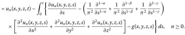
We construct an iteration formula by applying Eqs. (1.1) and (2.1) as follows:
un+1(x,y,z,t)
So the VIM with an auxiliary parameter is defined as
unknown suitableh. In order to find a proper value forhto obtain an accurate approximate solution, we define the following residual function:
rN(x,y,z,t,h)
and the following error of norm two of the residual function:
eN(h) =
Now we apply a numerical integration scheme to calculateeN(h), approximately. Note that
the optimal value ofhminimizes the norm two of the residual function.
4 Convergence of the proposed method
Now we investigate the convergence of the proposed method for three-dimensional equa-tion. In the sequel, the linear operator isL=∂∂t. Also, we define the operatorFas follows:
Moreover, the recurrence scheme can be defined as follows:
⎧ ⎨ ⎩
v0(x,y,z,t) =u0(x,y,z,t),
s0(x,y,z,t) =v0(x,y,z,t),
and
⎧ ⎨ ⎩
v1(x,y,z,t,h) =Fs0(x,y,z,t),
s1(x,y,z,t,h) =s0(x,y,z,t) +v1(x,y,z,t,h),
and in general forn≥1,
⎧ ⎨ ⎩
vn+1(x,y,z,t,h) =Fsn(x,y,z,t,h),
sn+1(x,y,z,t,h) =sn(x,y,z,t,h) +vn+1(x,y,z,t,h).
(4.2)
Consequently we have
u(x,y,z,t,h) = lim
n→∞sn(x,y,z,t,h) =v0(x,y,z,t) +
∞
n=1
vn(x,y,z,t,h). (4.3)
The initial approximationu0(x,y,z,t) can be freely chosen and the only restriction is
satis-faction of the given initial conditions defined in (2) withLu0(x,y,z,t) = 0. For the
approx-imation purpose, the solutionu(x,y,z,t,h) =v0(x,y,z,t) +∞n=1vn(x,y,z,t,h) is
approxi-mated by theNth-order truncated seriesuN(x,y,z,t,h) =v0(x,y,z,t) +
N
n=1vn(x,y,z,t,h).
The approximate solutionuN(x,y,z,t,h) contains the auxiliary parameterh. It is the
aux-iliary parameter which ensures that the assumption can be satisfied by means of the error of norm two of the residual function. The following theorems provide the sufficient con-ditions for convergence and validity of the proposed method.
Theorem 4.1 Let H be a real Hilbert space andFbe an operator on H.If there is h∗= 0
and0 <ξ< 1such that
⎧ ⎪ ⎪ ⎨ ⎪ ⎪ ⎩
Fs0(x,y,z,t) ≤ξs0(x,y,z,t),
Fs1(x,y,z,t,h∗) ≤ξFs0(x,y,z,t),
Fsn(x,y,z,t,h∗) ≤ξFsn–1(x,y,z,t,h∗), n= 2, 3, . . . ,
(4.4)
then the series solution defined in(4.3)with
u(x,y,z,t,h) = lim
n→∞sn
x,y,z,t,h∗=v0(x,y,z,t) + ∞
n=1
vn
x,y,z,t,h∗ (4.5)
converges.
Proof The proof is straightforward by noting the proof of Theorem 4.1 in [53].
Theorem 4.2 LetL= ∂
∂t. If we have u(x,y,z,t) =v0(x,y,z,t) +
∞
n=1vn(x,y,z,t,h∗),then
u(x,y,z,t),is the exact solution of the problem(1.1).
Proof The proof is straightforward by noting the proof of Theorem 4.2 in [53].
Theorem 4.3 Suppose that the series solution u(x,y,z,t) =v0(x,y,z,t) +
∞
n=1vn(x,y,z,t,
series uN(x,y,z,t) =v0(x,y,z,t) +
N
n=1vn(x,y,z,t,h∗),is used as an approximate solution,
then the maximum error is estimated as
u(x,y,z,t) –uN(x,y,z,t)≤
1 1 –ξξ
N+1v 0.
Proof The proof is straightforward by noting the proof of Theorem 4.3 in [53].
5 Numerical examples
In this section, some test problems are provided to investigate the practical computational efficiency and reliability of the proposed method.
Example1 Consider the following three-dimensional modified anomalous fractional sub-diffusion equation:
∂u(x,y,z,t) ∂t
=
∂1–α ∂t1–α+
∂1–β ∂t1–β +
∂1–γ ∂t1–γ
∂2u(x,y,z,t) ∂x2 +
∂2u(x,y,z,t) ∂y2 +
∂2u(x,y,z,t) ∂z2
+g(x,y,z,t), (x,y,z,t)∈Ω, (5.1)
where
g(x,y,z,t) =sin(x+y+z)
(1 +α+β+γ)tα+β+γ + 3Γ(2 +α+β+γ) Γ(1 + 2α+β+γ)t
2α+β+γ
+ 3Γ(2 +α+β+γ) Γ(1 +α+ 2β+γ)t
α+2β+γ+ 3 Γ(2 +α+β+ϑ) Γ(1 +α+β+ 2ϑ)t
α+β+2ϑ
,
with the initial condition u(x,y,z, 0) = 0, which admits the exact solutionu(x,y,z,t) =
t1+α+β+γsin(x+y+z).
TakeΩ= [0, 8π]×[0, 8π]×[0, 8π]×[0, 2]. According to the standard VIM, we have the following variational iteration formula:
un+1(x,y,z,t)
=un(x,y,z,t) –
t
0
∂un(x,y,z,s)
∂s –
∂1–α ∂s1–α +
∂1–β ∂s1–β +
∂1–γ ∂s1–γ
×
∂2un(x,y,z,s)
∂x2 +
∂2un(x,y,z,s)
∂y2 +
∂2un(x,y,z,s)
∂z2
–g(x,y,z,s)
ds, n≥0.
By starting the solution procedure from u0(x,y,z,t) =u(x,y,z, 0) = 0, we may stop at
u7(x,y,z,t). The graphs of the approximate solution and the absolute error function of
u7(x, 8π, 8π,t) for (x,t)∈[0, 8π]×[0, 2] and (α=β=14,γ =12) are shown in Figs.1and2
(left side), respectively. Also, the graphs of the absolute error function ofu7(x, 8π, 8π, 0.5)
andu7(x, 8π, 8π, 1.5) forx∈[0, 8π] are shown in Figs.3 and4 (left side), respectively.
From these figures it can be seen thatu7(x,y,z,t) is not accurate for the large values ofx,
y,zandt. Now, by applying the recurrence scheme (3.3), we successively have
Figure 1The graphs of the approximate solutionu(x, 8π, 8π,t) for Example1via the standard VIM (left side) and the upgraded VIM withh= 0.18 as an auxiliary parameter (right side) in the case (α=β=14,γ=12)
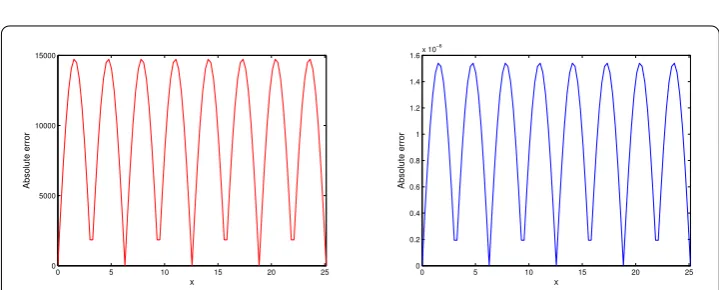
Figure 2The graphs of the absolute error function ofu(x, 8π, 8π,t) for Example1via the standard VIM (left side) and the upgraded VIM withh= 0.18 as an auxiliary parameter (right side) in the case (α=β=14,γ=12)
Figure 3The graphs of the absolute error function ofu(x, 8π, 8π, 0.5) for Example1via the standard VIM (left side) and the upgraded VIM withh= 0.18 as an auxiliary parameter (right side) in the case (α=β=14,γ=12)
u1(x,y,z,t,h)
=hsin(x+y+z)
3Γ(2 +α+β+γ) Γ(2 + 2α+β+γ)t
1+2α+β+γ + 3Γ(2 +α+β+γ) Γ(2 +α+ 2β+γ)t
1+α+2β+γ
+ 3 Γ(2 +α+β+γ) Γ(2 +α+β+ 2γ)t
1+α+β+γ
+t1+α+β+2γ
Figure 4The graphs of the absolute error function ofu(x, 8π, 8π, 1.5) for Example1via the standard VIM (left side) and the upgraded VIM withh= 0.18 as an auxiliary parameter (right side) in the case (α=β=14,γ=12)
and in general
un+1(x,y,z,t,h)
=un(x,y,z,t,h) –h
t
0
∂un(x,y,z,s,h)
∂s –
∂1–α ∂s1–α +
∂1–β ∂s1–β +
∂1–γ ∂s1–γ
×
∂2u
n(x,y,z,s,h)
∂x2 +
∂2u
n(x,y,z,s,h)
∂y2 +
∂2u
n(x,y,z,s,h)
∂z2
–g(x,y,z,s)
ds,
n≥1.
In order to find a proper value forhto obtain an accurate approximate solution of (5.1), we define the following residual function:
r7(x,y,z,t,h)
=∂u7(x,y,z,t,h) ∂t –
∂1–α ∂t1–α +
∂1–β ∂t1–β+
∂1–γ ∂t1–γ
×
∂2u
7(x,y,z,t,h)
∂x2 +
∂2u
7(x,y,z,t,h)
∂y2 +
∂2u
7(x,y,z,t,h)
∂z2
–g(x,y,z,t),
and the following error defined based on the norm two of residual function:
e7(h) =
2
0 8π
0 8π
0 8π
0
r27(x,y,z,t,h)dx dy dz dt
1
2
.
The minimum point ofe7(h) when (α=β=41,γ=12) is obtained ath0.18 by using Maple
software. Substitutingh= 0.18 inu7(x, 8π, 8π,t,h), reduces the absolute error of the
7th-step remarkably. The graphs of the approximate solution and the absolute error functions ofu7(x, 8π, 8π,t, 0.18) for (x,t)∈[0, 8π]×[0, 2] are shown in Figs.1(right side) and2(right
side), respectively. Also, the graphs of the absolute error functions ofu7(x, 8π, 8π, 0.5, 0.18)
andu7(x, 8π, 8π, 1.5, 0.18) forx∈[0, 8π] are shown in Figs.3and4(right side),
respec-tively. These figures imply thatu7(x,y,z,t, 0.18) is a highly accurate approximate solution
Example2 Consider the following three-dimensional modified anomalous fractional sub-diffusion equation:
∂u(x,y,z,t) ∂t
=
1 π2
∂1–α ∂t1–α+
1 π2
∂1–β ∂t1–β +
1 π2
∂1–γ ∂t1–γ
×
∂2u(x,y,z,t) ∂x2 +
∂2u(x,y,z,t) ∂y2 +
∂2u(x,y,z,t) ∂z2
+g(x,y,z,t), (x,y,z,t)∈[0, 40]×[0, 40]×[0, 40]×[0, 2], (5.2)
where
g(x,y,z,t) =cosπ(x+y+z)2t+ 6 t
1+α
Γ(2 +α)+ 6
t1+β Γ(2 +β)+ 6
t1+γ Γ(2 +γ)
,
with the initial conditionu(x,y,z, 0) = 0, and the exact solutionu(x,y,z,t) =cos(π(x+y+
z))t2.
According to the standard VIM, we have the following variational iteration formula:
un+1(x,y,z,t)
=un(x,y,z,t) –
t
0
∂un(x,y,z,s)
∂s –
1 π2
∂1–α ∂s1–α +
1 π2
∂1–β ∂s1–β +
1 π2
∂1–γ ∂s1–γ
×
∂2un(x,y,z,s)
∂x2 +
∂2un(x,y,z,s)
∂y2 +
∂2un(x,y,z,s)
∂z2
–g(x,y,z,s)
ds, n≥0.
By starting the solution procedure fromu0(x,y,z,t) =u(x,y,z, 0) = 0, we may repeat until
to computeu7(x,y,z,t). The graphs of the approximate solution and the absolute error
functions ofu7(x, 40, 40,t) for (x,t)∈[0, 40]×[0, 2] and (α= 14,β=12,γ =34) are shown
in Figs.5(left side) and6(left side), respectively. Also, the graphs of the absolute error functions ofu7(x, 40, 40, 0.5) andu7(x, 40, 40, 1.5) forx∈[0, 40] are, respectively, shown in
Figs.7and8(left side). It can be seen thatu7(x,y,z,t) is not accurate for large values ofx,
y,zandt. Now, by using the recurrence formula defined in (3.3), we successively have
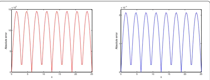
Figure 6The graphs of the absolute error function ofu(x, 40, 40,t) for Example2via the standard VIM (left side) and the upgraded VIM withh= 0.18 as an auxiliary parameter (right side) in the case
(α=14,β=12,γ=34)
Figure 7The graphs of the absolute error function ofu(x, 40, 40, 0.5) for Example2via the standard VIM (left side) and the upgraded VIM withh= 0.18 as an auxiliary parameter (right side) in the case
(α=14,β=12,γ=34)
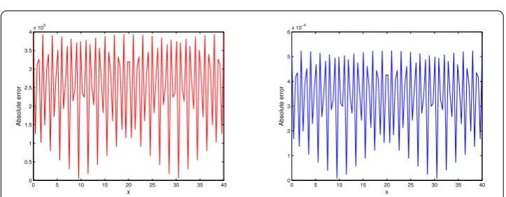
Figure 8The graphs of the absolute error function ofu(x, 40, 40, 1.5) for Example2via the standard VIM (left side) and the upgraded VIM withh= 0.18 as an auxiliary parameter (right side) in the case
(α=14,β=12,γ=34)
u0(x,y,z,t) =u(x,y,z, 0) = 0,
u1(x,y,z,t,h) =hcos
π(x+y+z)6 t
2+α
Γ(3 +α)+ 6
t2+β Γ(3 +β)+ 6
t2+γ Γ(3 +γ)+t
2
and in general
In order to find a proper value forhwhich leads to the accurate approximation, we define the following residual function:
and the following error of norm two of residual function:
e7(h) =
Maple software. Substitutingh= 0.18 inu7(x, 40, 40,t,h), remarkably reduces the absolute
error of approximation method. The graphs of the approximate solution and the abso-lute error functions ofu7(x, 40, 40,t, 0.18) for (x,t)∈[0, 40]×[0, 2] are shown in Figs.5
(right side) and 6 (right side), respectively. The graphs of the absolute error functions ofu7(x, 40, 40, 0.5, 0.18) andu7(x, 40, 40, 1.5, 0.18) forx∈[0, 40] are respectively shown in
Figs.7and8(right side). The demonstrated figures reveal thatu7(x,y,z,t, 0.18) is the highly
accurate approximate solution even for the large values ofx,y,zandt.
6 Conclusion
Funding
Zakieh Avazzadeh wishes to express gratitude to the Natural Science Foundation of Jiangsu Province (Grant No. BK20150964) and the National Natural Science Foundation of China (Grant No. 11671210).
Competing interests
The authors declare that they have no competing interests.
Authors’ contributions
All authors contributed equally to the writing of this paper. All authors read and approved the final manuscript.
Author details
1School of Mathematics and Physics, West Yunnan University, Yunnan, China.2Department of Mathematics, Shiraz
University of Technology, Shiraz, Iran.3School of Mathematical Sciences, Nanjing Normal University, Nanjing, China. 4Engineering School (DEIM), University of Tuscia, Viterbo, Italy.
Publisher’s Note
Springer Nature remains neutral with regard to jurisdictional claims in published maps and institutional affiliations.
Received: 19 February 2019 Accepted: 19 August 2019 References
1. Podlubny, I.: Fractional Differential Equations. Academic Press, New York (1999)
2. Meerschaert, M.M., Benson, D., Baeumer, B.: Operator Lévy motion and multiscaling anomalous diffusion. Phys. Rev. E 63, 1112–1117 (2001)
3. Solomon, T.H., Weeks, E.R., Swinney, H.L.: Observations of anomalous diffusion and Lévy flights in a 2-dimensional rotating flow. Phys. Rev. Lett.71, 3975–3979 (1993)
4. Yuste, S.B., Lindenberg, K.: Subdiffusion-limitedA+Areactions. Phys. Rev. Lett.87, 118301 (2001)
5. Raberto, M., Scalas, E., Mainardi, F.: Waiting-times and returns in high-frequency financial data: an empirical study. Physica A314, 749–755 (2002)
6. Mainardi, F., Raberto, M., Gorenflo, R., Scalas, E.: Fractional calculus and continuous-time finance II: the waiting-time distribution. Physica A287, 468–481 (2000)
7. Benson, D.A., Wheatcraft, S.W., Meerschaert, M.M.: Application of a fractional advection?dispersion equation. Water Resour. Res.36, 1403–1412 (2000)
8. Ren, J., Sun, Z., Zhao, X.: Compact difference scheme for the fractional sub-diffusion equation with Neumann boundary conditions. J. Comput. Phys.232, 456–467 (2013)
9. Tayebi, A., Shekari, Y., Heydari, M.H.: A meshfree approach for solving 2D variable-order fractional nonlinear diffusion-wave equation. Comput. Methods Appl. Mech. Eng.350, 154–168 (2019)
10. Heydari, M.H., Avazzadeh, Z., Yang, Y.: A computational method for solving variable-order fractional nonlinear diffusion-wave equation. Appl. Math. Comput.352, 235–248 (2019)
11. Heydari, M.H., Hooshmandasl, M.R., Cattani, C., Hariharan, G.: An optimization wavelet method for multi variable-order fractional differential equations. Fundam. Inform.153(3–4), 173–198 (2017)
12. Heydari, M.H., Avazzadeh, Z., Farzi Haromi, M.: A wavelet approach for solving multi-term variable-order time fractional diffusion-wave equation. Appl. Math. Comput.341, 215–228 (2019)
13. Heydari, M.H., Avazzadeh, Z.: Legendre wavelets optimization method for variable-order fractional Poisson equation. Chaos Solitons Fractals112, 180–190 (2018)
14. Heydari, M.H., Avazzadeh, Z.: A new wavelet method for variable-order fractional optimal control problems. Asian J. Control20(5), 1–14 (2018)
15. Heydari, M.H., Avazzadeh, Z.: An operational matrix method for solving variable-order fractional biharmonic equation. Comput. Appl. Math.37(4), 4397–4411 (2018)
16. Heydari, M.H.: A new direct method based on the Chebyshev cardinal functions for variable-order fractional optimal control problems. J. Franklin Inst.355, 4970–4995 (2018)
17. Hajipour, M., Jajarmi, A., Baleanu, D., Sun, H.G.: On an accurate discretization of a variable-order fractional reaction–diffusion equation. Commun. Nonlinear Sci. Numer. Simul.69, 119–133 (2019)
18. Baleanu, D., Jajarmi, A., Asad, J.H.: Classical and fractional aspects of two coupled pendulums. Rom. Rep. Phys.71(1), 103 (2019)
19. Baleanu, D., Sadat, S., Jajarmi, A., Asad, J.H.: New features of the fractional Euler–Lagrange equations for a physical system within non-singular derivative operator. Eur. Phys. J. Plus134, 181 (2019)
20. Baleanu, D., Asad, J.H., Jajarmi, A.: New aspects of the motion of a particle in a circular cavity. Proc. Rom. Acad., Ser. A: Math. Phys. Tech. Sci. Inf. Sci.19(2), 361–367 (2018)
21. Metzler, R., Klafter, J.: The random walk’s guide to anomalous diffusion: a fractional dynamics approach. Phys. Rep. 339, 1–77 (2000)
22. Kilbas, A., Srivastava, H., Trujillo, J.: Theory and Applications of Fractional Differential Equations. Elesvier, Boston (2006) 23. Schneider, W., Wyss, W.: Fractional diffusion and wave equations. J. Math. Phys.30, 134–144 (1989)
24. Mainardi, F.: The fundamental solutions for the fractional diffusion-wave equation. Appl. Math. Lett.9, 23–28 (1996) 25. Gorenflo, R., Iskenderov, A., Luchko, Y.: Mapping between solutions of fractional diffusion-wave equations. Fract. Calc.
Appl. Anal.3, 75–86 (2000)
26. Agrawal, O.: Solution for a fractional diffusion-wave equation defined in a bounded domain. Nonlinear Dyn.29, 145–155 (2002)
27. Huang, F., Liu, F.: The time fractional diffusion and advection–dispersion equation. ANZIAM J.46, 317–330 (2005) 28. Yuste, S., Acedo, L.: An explicit finite difference method and a new von Neumann-type stability analysis for fractional
29. Yuste, S.: Weighted average finite difference methods for fractional diffusion equations. J. Comput. Phys.216, 264–274 (2006)
30. Sun, Z., Wu, X.: A fully discrete difference scheme for a diffusion-wave system. Appl. Numer. Math.56, 193–209 (2006) 31. Chen, C., Liu, F., Turner, I., Anh, V.: A Fourier analysis method for the fractional diffusion equation describing
sub-diffusion. J. Comput. Phys.227, 886–897 (2007)
32. Li, X., Xu, C.: A space-time spectral method for the time fractional diffusion equation. SIAM J. Numer. Anal.47, 2108–2131 (2009)
33. Abbaszadeh, M., Mohebbi, A.: A fourth-order compact solution of the two-dimensional modified anomalous fractional sub-diffusion equation with a nonlinear source term. Comput. Math. Appl.66, 1345–1359 (2013) 34. Heydari, M.H., Hooshmandasl, M.R., Ghaini, F.M.M., Cattani, C.: Wavelets method for the time fractional diffusion-wave
equation. Phys. Lett. A379, 71–76 (2015)
35. Mohebbi, A., Abbaszadeh, M., Dehghan, M.: Solution of two-dimensional modified anomalous fractional sub-diffusion equation via radial basis functions (RBF) meshless method. Eng. Anal. Bound. Elem.38, 72–82 (2014) 36. Heydari, M.H., Hooshmandasl, M.R., Cattani, C.: Numerical solution of fractional sub-diffusion and time-fractional
diffusion-wave equations via fractional-order Legendre functions. Eur. Phys. J. Plus131, 268–290 (2016)
37. Zhuang, P., Liu, F.: Implicit difference approximation for the two-dimensional space-time fractional diffusion equation. J. Appl. Math. Comput.25, 269–282 (2007)
38. Zhuang, P., Liu, F.: Finite difference approximation for two-dimensional time fractional diffusion equation. J. Algorithms Comput. Technol.1(1), 1–15 (2007)
39. Liu, Q., Gu, Y., Zhuang, P., Liu, F., Nie, Y.: An implicit RBF meshless approach for time fractional diffusion equations. Comput. Mech.48(1), 1–12 (2001)
40. Chen, C., Liu, F., Turner, I., Anh, V.: Numerical schemes and multivariate extrapolation of a two-dimensional anomalous sub-diffusion equation. Numer. Algorithms54, 1–21 (2010)
41. Zhang, Y., Sun, Z.: Alternating direction implicit schemes for the two-dimensional fractional sub-diffusion equation. J. Comput. Phys.230, 8713–8728 (2011)
42. He, J.: Variational iteration method—a kind of nonlinear analytical technique: some examples. Int. J. Non-Linear Mech.34, 699–708 (1999)
43. Inokuti, M., Sekine, H., Mur, T.: General Use of the Lagrange Multiplier in Nonlinear Mathematical Physics. Pergamon, New York (1978)
44. Herisanu, N., Marinca, V.: A modified variational iteration method for strongly nonlinear problems. Nonlinear Sci. Lett. A, Math. Phys. Mech.1(2), 183–192 (2010)
45. Noor, M.A., Mohyud-Din, S.: Variational iteration method for solving higher-order nonlinear boundary value problems using He’s polynomials. Int. J. Nonlinear Sci. Numer. Simul.9(2), 141–156 (2008)
46. Yilmaz, E., Inc, M.: Numerical simulation of the squeezing flow between two infinite plates by means of the modified variational iteration method with an auxiliary parameter. Nonlinear Sci. Lett. A, Math. Phys. Mech.1(3), 297–306 (2010) 47. Wu, G.C., Baleanu, D.: Variational iteration method for fractional calculus—a universal approach by Laplace transform.
Adv. Differ. Equ.2013, 18 (2013)
48. Wu, G.C., Baleanu, D.: New applications of the variational iteration method—from differential equations to
q-fractional difference equations. Adv. Differ. Equ.2013, 21 (2013)
49. Herisanu, N., Marinca, V.: A modified variational iteration method for strongly nonlinear problems. Nonlinear Sci. Lett. A, Math. Phys. Mech.1(2), 183–192 (2010)
50. Hosseini, M.M., Mohyud-Din, S., Ghaneai, H., Usman, M.: Auxiliary parameter in the variational iteration method and its optimal determination. Int. J. Nonlinear Sci. Numer. Simul.11(7), 495–502 (2010)
51. Hosseini, M., Mohyud-Din, S., Ghaneai, H.: Variational iteration method for nonlinear age-structured population models using auxiliary parameter. Z. Naturforsch. A65(12), 11–37 (2010)
52. Hosseini, M.M., Mohyud-Din, S., Ghaneai, H.: Variational iteration method for Hirota–Satsuma coupled KdV equation using auxiliary parameter. Int. J. Numer. Methods Heat Fluid Flow22(3), 277–286 (2012)
53. Ghaneai, H., Hosseini, M.M.: Variational iteration method with an auxiliary parameter for solving wave-like and heat-like equations in large domains. Comput. Math. Appl.65(9), 363–373 (2015)
54. Hajipour, M., Jajarmi, A., Baleanu, D.: On the accurate discretization of a highly nonlinear boundary value problem. Numer. Algorithms79(3), 679–695 (2018)