A fourth order accurate difference Dirichlet problem for the approximate solution of Laplace’s equation with integral boundary condition

R E S E A R C H

Open Access

A fourth-order accurate difference Dirichlet

problem for the approximate solution of

Laplace’s equation with integral boundary

condition

Adiguzel Dosiyev

1*

_{and Rifat Reis}

1

*_{Correspondence:}

[email protected]

1_{Department of Mathematics, Near}

East University, Nicosia, via Mersin 10, TRNC, Turkey

Abstract

A new constructive method for the finite-difference solution of the Laplace equation with the integral boundary condition is proposed and justified. In this method, the approximate solution of the given problem is defined as a sequence of 9-point solutions of the local Dirichlet problems. It is proved that when the exact solution u(x,y) belongs to the Hölder calssesC4,λ, 0 <

λ

< 1, on the closed solution domain, the uniform estimate of the error of the approximate solution is of orderO(h4_{), wherehis}

the mesh step. Numerical experiments are given to support analysis made.

Keywords: Finite difference method; Nonlocal integral boundary condition; Laplace’s equation; Uniform error

1 Introduction

Different finite-difference problems as approximations of the nonlocal problems with in-tegral boundary condition have been studied by many authors (see [1–5] and references given therein). They all were basically focusing on the following difficulties related to the existence of a quadrature approximation of the integral condition on the side of the do-main where nonlocal condition was given: (i) finding an approximate solution by solving the obtained system of equations which are non-band matrices, (ii) determining the rate of convergence of the approximate solution by appropriate smoothness conditions on the given data. In [1], a system of finite difference equations for the Poisson problem has been studied for the spectrum of the matrix to apply an iterative method. Moreover, the author obtained some conditions, under which this system has a unique solution. In [2] and [3], for the error of approximate solution, the order of estimation ofO(h2_{) in the differenceW}1 2

metric is obtained, wherehis the mesh step. In [4], the radial basis function collocation technique is used to find an approximate solution of an elliptic equation with nonlocal in-tegral boundary condition. In [5], a finite-difference approximation for the problem with integral boundary conditions is constructed by reducing the given problem to the prob-lem with nonlocal conditions containing derivatives. The authors proved that when the fourth-order partial derivatives of the exact solution are continuous on the closed

tion domain, the uniform estimate of orderO(h2_{|lnh|) is obtained for the error of the}

approximate solution.

In this paper, we propose and justify a new constructive method to solve a system of non-local 9-point finite-difference problem for the Laplace equation with the integral boundary condition. The solution of this nonlocal difference problem is defined as a solution of the 9-point Dirichlet problem by constructing approximate values of the solution on the side where the integral condition was given. Therefore, the approximate solution is obtained by solving a system with 9 diagonal matrices, for the realization of which many fast al-gorithms have been proposed (see [6,7]). Moreover, the uniform estimate of the error of approximate solution is of orderO(h4_{) when the given boundary functions on the sides}

be-long to the Hölder classesC4,λ_{, 0 <λ< 1. Finally, numerical experiments are demonstrated} to support the theoretical results.

The proposed method with the 5-point scheme was announced in [8].

Other nonlocal boundary value problems are stated and developed in numerous papers (see [9–20] and references therein).

2 Nonlocal boundary value problem

Let

R=(x,y) : 0 <x<a, 0 <y<b

be an open rectangle,γm_{,m= 1, 2, 3, 4, be its sides including the endpoints, numbered in}

the clockwise direction, beginning with the side lying on they-axis, and letγ =4_m=1γm

be the boundary ofRandR=R∪γ. LetC0denote the linear space of continuous functions of one variablexon the interval [0,a] of thex-axis, and vanishing at the pointsx= 0 and

x=a. For a functionf∈C0_{, we define the norm}

fC0=max 0≤x≤af(x).

It is clear that the spaceC0_{with this norm is complete.}

Consider the following nonlocal boundary value problem:

u= 0 onR, u= 0 onγ1∪γ3, u=τ onγ2, (1)

u(x, 0) =α

b

ξ

u(x,y)dy+μ(x), 0 <x<a, 0 <ξ<b, (2)

where ≡∂2_/∂x2_+∂2_/∂x2 _{is the Laplacian,τ =τ(x) and μ=μ(x) are given functions}

which belong toC0_{, andαis a given constant which satisfies the following inequality:}

|α|< 1

b–ξ. (3)

3 Nonlocal finite-difference problem and its reduction to the Dirichlet problem

We define a square mesh with sizeh=_Na =_Mb∗, whereN,M∗> 2 are integers, constructed

with the linesx,y=h, 2h, . . . . LetDhbe the set of nodes of this square grid and letRh=

R∩Dh,Rh=R∩Dh. We putγ_hm=γm_{∩Dh,m= 1, 2, 3, 4, andγ} h=

4

Let

[0,a]h=

x=xi,xi=ih,i= 0, 1, . . . ,N,h= a

N

be the set of points divided by the step sizehon [0,a]. LetC0

h be the linear space of grid functions defined on [0,a]h that vanish atx= 0 and x=a. The norm of a functionfh∈C0

h is defined as

fhC0

h=x∈max[0,a]h

|fh|.

We introduce the operatorBhby

Buh(x,y)≡ u(x+h,y) +u(x–h,y) +u(x,y+h) +u(x,y–h)/5

+ u(x+h,y+h) +u(x+h,y–h) +

+u(x–h,y+h) +u(x–h,y–h)/20.

For the approximate solution of the nonlocal problem (1)–(2), we consider a solution of the following system of difference equations (see [1]):

uh=Buh onRh, uh= 0 onγ_h1∪γ_h3, uh=τh onγh2, (4)

uh(x, 0) =α

M

k=1

ρkuh(x,ηk) +μh onγh4, (5)

where equation (5) is obtained by approximating the integral in (2) and using Simpson’s rule withρ1=ρM=₃h,ρj=h₃(3 + (–1)j) forj= 2, 3, . . . ,M– 1,ηj=ξ+ (j– 1)h,j= 1, 2, . . . ,M, h= a

N, (M– 1)h+ξ=b,μhis the trace ofμonγ

4

h, and

ξ

his an integer.

We reduce a solution of the nonlocal differential problem to the solution of the local Dirichlet problem.

Letvhbe the solution of the finite-difference Dirichlet problem

vh=Bvh onRh, vh=τh onγh2, vh= 0 onγh/γh2, (6)

and we put

ϕi,h(x) =vh(x,ηi), i= 1, 2, . . . ,M, (7)

whereτhis the trace ofτ onγ_h2.

Letwhbe a solution of the following finite difference Dirichlet problem:

wh=Bwh onRh, wh= 0 onγh/γh4, wh=fh onγh4, (8)

wherefh∈Ch0, is an arbitrary function.

We define a linear operatorBh

i fromCh0toCh0as follows:

Bh_ifh(x) =wh(x,ηi), i= 1, 2, . . . ,M, (9)

Let

w∗_h(x,y) = 1

bfhCh0(b–y) onRh.

We have

wh(x,y)≤w∗_h(x,y), (x,y)∈γh. (10)

Sincew∗_h=Bw∗_honRh, from (9)–(10) and by a comparison theorem (see [21, Chap. 4]),

we have

Bh_ifh_C0

h≤ fh_C0

h

1 –ξ+ (i– 1)h

b

, i= 1, 2, . . . ,M, (11)

and then for the norm of operatorBh i, we get

Bh_i< 1, i= 1, 2, . . . ,M. (12)

Let

ϕh=α M

k=1

ρkϕk,h(x), x∈[0,a]h, (13)

whereϕk,h(x) is the function from (7).

In the view of inequality (3), we have

|α|

M

k=1

ρk=q0< 1. (14)

Inequalities (12) and (14) yield

q0Bh1=q< 1. (15)

Lemma 1 A solution of the finite difference problem(4)–(5)can be represented as

uh=vh+wh, (16)

where vhis the solution of problem(6)and whis the solution of problem(8)withfhbeing a solution of the following nonlinear equation:

fh=ϕh+μh+α M

k=1

ρkBh_kfh onγ_h4. (17)

From (13) and (17), it follows that

Thus, the unknown function onγ_h4in problem (8) is a solution of the nonlinear equation (17).

Theorem 2 There exists a unique solutionfhof the nonlinear equation(17).

Proof Consider the following sequences inC0

h:

From this, for the positive integersmandnwithm>n, we get

Applying inequality (11), we reach

ψ_im_,h–ψ_in_,hC0

h≤q

ψ_im_,h–1–ψ_in_,h–1_C0

h, (19)

whereqis defined by (15). In a similar way, from (19) we obtain

ψ_im_,h–ψ_in_,hC0

which shows that sequences (18) are Cauchy. SinceC_h0is complete, there are limits

lim n→∞ψ

n

By using (11) and (15),

In view of relations (17) and (22), we obtain a solution of the nonlinear equation (17) as

fh=ϕh+μh+α

Then, we obtain the following inequality:

fh,1–fh,2C_h0=

4 Convergence of the finite-difference problem

We say that F∈Ck,λ_{(E), ifF haskth derivatives onE satisfying Hölder condition with}

Hence, for the approximate solution of the nonlocal problem (1)–(2), we define the fol-lowing difference problem:

un_h=Bhun_h onRh, un_h=τh onγh2, unh= 0 onγh1∪γh3, (24) un_h=f_hn onγ_h4. (25)

Theorem 3 The following estimate holds:

whereun_h is a solution of problem(24)–(25),u is the exact solution of nonlocal boundary value problem(1)–(2),c1and c∗are constants independent of h,q0is defined by(14),and

q1= 1 –ξ_b.

Proof LetUbe the exact solution of the system of the following problem:

U= 0 onR, U=τ onγ2, U= 0 onγ1∪γ3, (27)

U(x, 0) =α

M

k=1

ρkU(x,ηk) +μ(x), 0≤x≤a. (28)

LetVbe a solution of the Dirichlet problem

V= 0 onR, V=τ onγ2, V= 0 onγ/γ2, (29)

and denote by

ϕk(x) =V(x,ηk) fork= 1, 2, . . . ,M, (30)

whereηk=ξ+ (k– 1)h,k= 1, 2, . . . ,M. We define the function

ϕ=α

M

k=1

ρkϕk. (31)

Consider the Dirichlet problem

W= 0 onR, W= 0 onγ/γ4, W=f onγ4, (32)

wheref is an unknown function fromC0_{. The linear operatorBi:C}0_→C0_{is defined as}

Bif(x) =W(x,ηi)∈C0, i= 1, 2, . . . ,M.

Then following inequality holds for the norm|Bi|:

|Bi|<

1 –ξ+ (i– 1)h

b

, i= 1, 2, . . . ,M.

By analogy with the results in [18], it is shown that a solutionUof problem (27)–(28) can be represented asU=V+WwhereVandW are the solutions of problem (29) and (32), respectively, whenf is defined by

f =ϕ+μ+α

M

k=1

ρkψk. (33)

Here the functions ψ1,ψ2, . . . ,ψM are fromC0, and are defined as the solutions of the

nonlinear equations

ψi=Bi

ϕ+μ+α

M

k=1

ρkψk

Therefore, the nonlocal problem (27)–(28) is reduced to the following Dirichlet problem:

U= 0 onR, U=τ onγ2, U= 0 onγ1∪γ3, (35)

U(x, 0) =f, 0≤x≤a, (36)

wheref is defined by (33). The solutionψi,i= 1, 2, . . . ,M, of system (34) is found as a limit

of the infinite sequence of functions{ψ_in}∞_n

=0inC

0_{defined by}

ψ_i0= 0, ψ_in=Bi

ϕ+μ+α

M

k=1

ρkψkn–1

,

i= 1, 2, . . . ,M;n= 1, 2, . . . . (37)

Sinceτ(x) in (29) belongs toC4,λ_(γ2_{) andτ}(2m)_{(0) =τ}(2m)_{(a) = 0,m= 0, 1, 2, it follows from}

[22] that

max

(x,y)∈Rh|

vh–Vh| ≤c2h4, (38)

wherevhis a solution of problem (6),Vhis the trace of the solution of (29) onRhandc2is

a constant independent ofh. Letϕh,ψi,h, andψin,hbe the trace ofϕ,ψi, andψinon [0,a]h,

respectively, and let (Bi(F))hbe the trace ofBi(F) on [0,a]hfor any functionF∈C4,λ[0,a].

By (7), (13), (30), (31), and (38), we obtain

ϕh–ϕhC_h0≤c3h4, (39)

where c3 is a constant independent ofh. By using (18) and (37), we have, for all i=

1, 2, . . . ,M,

ψ_i1_,h–ψ_i1_,hC0

h≤

Bh_i(ϕh–ϕh)_C0

h

+Bh_i(ϕh+μh) – Bi(ϕ+μ)

hC_h0. (40)

Applying (11) and (39), it follows that

Bh_i(ϕh–ϕh)_C0

h≤c4h

4_{, i= 1, 2, . . . ,M, (41)}

wherec4is a constant independent ofh. Similar to inequality (38), we have

Bh_i(ϕh+μh) – Bi(ϕ+μ)

hC_h0≤c5h

4_{, (42)}

wherec5is a constant independent ofh. From the relations (40)–(42), we have

ψ_i1_,h–ψ_i1_,h

C0_h≤c6h

wherec6is a constant independent ofh. Forn≥2, we have

By analogy with (54) in [20], it follows that

max

1≤k≤M

Bh_iψ_kn–1– Biψ_kn–1

hC_h0≤c7h

4_{, (45)}

wherec7is a constant independent ofh. From (45), we find that

wherec10andc11are constants independent ofh. According to (37), it follows that

ψ_in–ψ_in–1

C0≤ |Bi||α|

M

k=1

|ρk|ψin–1–ψin–2C0, i= 1, 2, . . . ,M, (50)

whereϕis defined by (31). From (49) and (50), we have

ψ_in–ψ_in–1

C0≤q1n ϕC0+μ_C0, i= 1, 2, . . . ,M,

whereq1= 1 –ξ_b. Moreover, for anym= 1, 2, . . . , we obtain

ψ_in+m–ψ_in_C0≤qn1+1

1 –qm1

1 –q1

ϕ_C0+μ_C0

, i= 1, 2, . . . ,M. (51)

Since

ψ_in–ψi_C0≤ψ_in+m–ψ_in_C0+ψ_in+m–ψi_C0, i= 1, 2, . . . ,M, (52)

by taking the limit asm→ ∞, from (51) and (52), it follows that

ψ_in–ψi_C0≤

qn1+1

1 –q1

ϕ_C0+μ_C0

, i= 1, 2, . . . ,M. (53)

From (48) and (53), we have

ψ_in_,h–ψi,h_C0

h≤c11h

4₊ qn1+1

1 –q1

ϕ_C0+μ_C0

, i= 1, 2, . . . ,M. (54)

LetUh(x,y) be the solution of the system of grid equations

Uh=BhUh onRh, Uh=τ onγh2, Uh= 0 onγh1∪γh3, (55)

Uh=fh onγ_h4, (56)

which approximates problem (35)–(36) whenfhis the trace off on [0,a]h. Sinceτ,μ,ϕ,

andψi,i= 1, 2, . . . ,M, belong toC4,λ, 0 <λ< 1, on the interval 0≤x≤1, and the (2m)th

order derivatives vanish at the endpoints form= 0, 1, 2 (see [20]), by [22], we have

max

(x,y)∈Rh|

Uh–U| ≤c12h4, (57)

whereUis the solution of problem (35)–(36) andc12is a constant independent ofh. In

view of inequalities (39) and (54), we obtain

f_hn–fh_C0

h≤c13h

4_+q 0

qn₁+1

1 –q1

ϕ_C0+μ_C0

, (58)

whereq0is defined by (14) andc13is a constant independent ofh. By the grid maximum

principle and from (58), we have

max

(x,y)∈Rh

un_h–Uh≤c13h4+q0

qn₁+1

1 –q1

ϕ_C0+μ_C0

whereun_his the solution of problem (24)–(25) andUhis the solution of problem (55)–(56). According to estimates (57) and (59), the following inequality holds:

max

whereUis the solution of problem (35)–(36) andc14is a constant independent ofh.

Using the estimate (60) and by the maximum principle for the Laplace equation with the truncation error of Simpson’s rule, which is order ofO(h4_{), we obtain the final estimate}

max

From (62) it follows that

Table 1 Solutions on the liney= 0 of Problem1

h= 1/16 h= 1/32 h= 1/64 h= 1/128

1.06874E–003 1.06873E–003 1.06874E–003 1.06877E–003

2.09641E–003 2.09639E–003 2.09641E–003 2.09647E–003

3.04351E–003 3.04350E–003 3.04352E–003 3.04361E–003

3.87366E–003 3.87364E–003 3.87366E–003 3.87378E–003

4.55494E–003 4.55491E–003 4.55495E–003 4.55508E–003

5.06118E–003 5.06115E–003 5.06119E–003 5.06134E–003

5.37292E–003 5.37289E–003 5.37293E–003 5.37309E–003

5.47818E–003 5.47815E–003 5.47819E–003 5.47835E–003

5.37292E–003 5.37289E–003 5.37293E–003 5.37309E–003

5.06118E–003 5.06115E–003 5.06119E–003 5.06134E–003

4.55494E–003 4.55491E–003 4.55495E–003 4.55508E–003

3.87366E–003 3.87364E–003 3.87366E–003 3.87378E–003

3.04351E–003 3.04350E–003 3.04352E–003 3.04361E–003

2.09641E–003 2.09639E–003 2.09641E–003 2.09647E–003

1.06874E–003 1.06873E–003 1.06874E–003 1.06877E–003

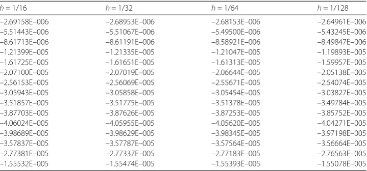
Table 2 Solutions on the liney= 0 of Problem2

h= 1/16 h= 1/32 h= 1/64 h= 1/128

–2.69158E–006 –2.68953E–006 –2.68153E–006 –2.64961E–006

–5.51443E–006 –5.51067E–006 –5.49500E–006 –5.43245E–006

–8.61713E–006 –8.61191E–006 –8.58921E–006 –8.49847E–006

–1.21399E–005 –1.21335E–005 –1.21047E–005 –1.19893E–005

–1.61725E–005 –1.61651E–005 –1.61313E–005 –1.59957E–005

–2.07100E–005 –2.07019E–005 –2.06644E–005 –2.05138E–005

–2.56153E–005 –2.56069E–005 –2.55671E–005 –2.54074E–005

–3.05943E–005 –3.05858E–005 –3.05454E–005 –3.03827E–005

–3.51857E–005 –3.51775E–005 –3.51378E–005 –3.49784E–005

–3.87703E–005 –3.87626E–005 –3.87253E–005 –3.85752E–005

–4.06024E–005 –4.05955E–005 –4.05620E–005 –4.04271E–005

–3.98689E–005 –3.98629E–005 –3.98345E–005 –3.97198E–005

–3.57837E–005 –3.57787E–005 –3.57564E–005 –3.56664E–005

–2.77381E–005 –2.77337E–005 –2.77183E–005 –2.76563E–005

–1.55532E–005 –1.55474E–005 –1.55393E–005 –1.55078E–005

The exact solutions of Problems1and2are unknown. The approximate values of Prob-lems1and2on the liney= 0 obtained by the proposed method are given in Tables1and2, respectively. According to repeated digits, for the decreasing mesh stepsh=₁₆1,₃₂1,₆₄1,₁₂₈1 , it follows that the maximum error on this line decreases asO(h4_{). To obtain these results,}

14 iterations are run for the construction off_hnwith the successive error which is less than 10–16.

Problem 3

u= 0 onR, u(0,y) =u(1,y) = 0, 0≤y≤2,

u(x, 2) =e2πsinπx, 0≤x≤1,

u(x, 0) = 1 100

2

1 16

u(x,y)dy+μ(x), 0 <x< 1,

whereu=eπy_{sinπxis the exact solution,μ(x) = [1 +}α π(1 –e2

Table 3 Maximum errors for the solution of Problem3

h Max error Order of reduction

1/16 1.40629393×10–9

1/32 8.77042882×10–11 _16.03449

1/64 5.47739631×10–12 _16.01203

1/128 3.42279360×10–13 _16.00270

Table 4 CPU times (in seconds) for Problem1

h Discrete Fourier Gauss–Seidel

with reducing

Gauss–Seidel without reducing

1/16 0.10125 0.13325 0.65250

1/32 1.58375 2.27125 6.70625

1/64 19.87500 25.15375 81.11175

1/128 284.72625 467.22025 1325.14725

Table 5 CPU times (in seconds) for Problem2

h Discrete Fourier Gauss–Seidel

with reducing

Gauss–Seidel without reducing

1/16 0.19115 0.23565 0.71300

1/32 2.00135 3.97115 8.12375

1/64 26.6875 37.35625 90.72425

1/128 355.62775 580.22315 1798.54315

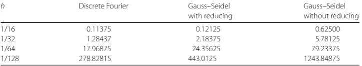
Table 6 CPU times (in seconds) for Problem3

h Discrete Fourier Gauss–Seidel

with reducing

Gauss–Seidel without reducing

1/16 0.11375 0.12125 0.62500

1/32 1.28437 2.18375 5.78125

1/64 17.96875 24.35625 79.23375

1/128 278.82815 443.0125 1243.84875

In Table3for Problem3, the maximum error for each steph=₂1k,k= 4, 5, 6, 7 and the

reduction orders are given. From the third column it follows that the convergence order isO(h4_).

In Tables4,5, and6, the results of the CPU times (in seconds), when solving Problems1, 2, and3, respectively, are given. In columns 2 and 3, the CPU times for the realization of the proposed approaches by the discrete Fourier method and by the Gauss–Seidel method are given. For the construction of the local functionf_hnfor Problems1and2, just 14 iterations are used. Problem3needs 11 iterations. In column 4, the Gauss–Seidel method is used to solve the given problems without reducing to the Dirichlet problem. From these results it follows that the discrete Fourier method, which cannot be used on the problem without reducing to the Dirichlet problem, is faster than others. The third and fourth columns show that for the method which is applicable for both approaches (as Gauss–Seidel), the CPU times with reducing are less than the CPU times without reducing to the Dirichlet problem.

6 Conclusion

A new constructive method for the approximate solution of the nonlocal boundary value for Laplace’s equation with integral boundary condition is given. In the proposed method, the system of finite-difference equations is defined as the 9-point solution of the Dirich-let problem by constructing the function on the side of the rectangle where the nonlocal boundary condition was given. This function is defined by using thenth term of the con-vergent simplest fixed point iteration (18) for the solution of the nonlinear system of (21). A uniform estimate for the error of the approximate solution of the nonlocal problem by using thenth term forn=max{[(lnh4(1 –q1))/lnq1], 1}is of orderO(h4), wherehis the

step size.

The proposed method gives an opportunity to solve nonlocal problems by using differ-ent fast algorithms constructed for the local Dirichlet problem by many authors (see [6] and the references therein).

Funding

Not applicable.

Competing interests

The authors declare that they have no competing interests.

Authors’ contributions

All authors contributed equally to the writing of this paper. All authors read and approved the final manuscript.

Publisher’s Note

Springer Nature remains neutral with regard to jurisdictional claims in published maps and institutional affiliations.

Received: 11 February 2019 Accepted: 1 August 2019 References

1. Sapagovas, M.P.: Difference method of increased order of accuracy for the Poisson equation with nonlocal conditions. Differ. Equ.44(7), 1018–1028 (2008)

2. Berikelashvili, G.K.: On the convergence of difference schemes for the third boundary value problem of elasticity theory. Comput. Math. Math. Phys.41(8), 1182–1189 (2001)

3. Berikelashvili, G.K., Khomeriki, N.: On the convergence of difference schemes for one nonlocal boundary value-problem. Lith. Math. J.52(4), 353–363 (2012)

4. Sajavicius, S.: Radial basis function method for a multidimensional linear elliptic equation with nonlocal boundary conditions. Comput. Math. Appl.67(7), 1407–1420 (2014)

5. Zhou, L., Yu, H.: Error estimate of a high accuracy difference scheme for Poisson equation with two integral boundary conditions. Adv. Differ. Equ.2018, 225 (2018)

6. Samarskii, A.A., Nikolaev, E.S.: Numerical Methods for Grid Equations, Vol. I, Direct Methods. Birkhäuser, Basel (1989) 7. Samarskii, A.A., Nikolaev, E.S.: Numerical Methods for Grid Equations, Vol. II, Iterative Methods. Birkhäuser, Basel (1989) 8. Dosiyev, A.A., Reis, R.: An approximate grid solution of a nonlocal boundary value problem with integral boundary

condition for Laplace’s equation. ITM Web Conf.22, 01016 (2018)

9. Bitsadze, A.V., Samarskii, A.A.: On some simplest generalizations of linear elliptic problems. Dokl. Akad. Nauk SSSR

185(4), 739–740 (1969)

10. Gurbanov, I.A., Dosiyev, A.A.: On the numerical solution of nonlocal boundary problems for quasilinear elliptic equations. In: Approximate Methods for Operator Equations, pp. 64–74. Baku State University, Baku (1984) 11. II’in, V.A., Moiseev, E.I.: Two-dimensional nonlocal boundary value problems for Poisson’s operator in differential and

difference variants. Math. Model.2, 139–150 (1990)

12. Gordeziani, N., Natalini, P., Ricci, P.E.: Finite-difference methods for solution of nonlocal boundary value problems. Comput. Math. Appl.50, 1333–1344 (2005)

13. Skubachevskii, A.L.: On necessary conditions for the Fredholm solvability of nonlocal elliptic equations. Proc. Steklov Inst. Math.260(1), 238–253 (2008)

14. Ashyralyev, A., Ozturk, E.: On Bitsadze–Samarskii type nonlocal boundary value problems for elliptic differential and difference equations. Well posedness. Appl. Math. Comput.219, 1093–1107 (2012)

15. Ashyralyev, A., Ozturk, E.: On a difference scheme of fourth order of accuracy for the Bitsadze–Samarskii type nonlocal boundary value problem. Math. Methods Appl. Sci.36, 936–955 (2013)

16. Volkov, E.A.: Approximate grid solution of a nonlocal boundary value problem for Laplace’s equation on a rectangle. Comput. Math. Math. Phys.53(8), 1128–1138 (2013)

17. Volkov, E.A., Dosiyev, A.A., Buranay, S.C.: On the solution of a nonlocal problem. Comput. Math. Appl.66, 330–338 (2013)

19. Volkov, E.A., Dosiyev, A.A.: On the numerical solution of a multilevel nonlocal problem. Mediterr. J. Math.13, 3589–3604 (2016)

20. Dosiyev, A.A.: Difference method of fourth order accuracy for the Laplace equation with multilevel nonlocal conditions. J. Comput. Appl. Math. (2018).https://doi.org/10.1016/j.cam.2018.04.046

21. Samarskii, A.A.: The Theory of Difference Schemes. Dekker, New York (2001)