Identification of source term for the ill posed Rayleigh–Stokes problem by Tikhonov regularization method

(1)

R E S E A R C H

Open Access

Identiﬁcation of source term for the ill-posed

Rayleigh–Stokes problem by Tikhonov

regularization method

Tran Thanh Binh

1

_{, Hemant Kumar Nashine}

2

_{, Le Dinh Long}

3

_{, Nguyen Hoang Luc}

4

_{and Can Nguyen}

5*

*_{Correspondence:} [email protected]

5_{Applied Analysis Research Group,}

Faculty of Mathematics and Statistics, Ton Duc Thang University, Ho Chi Minh City, Vietnam Full list of author information is available at the end of the article

Abstract

In this paper, we study an inverse source problem for the Rayleigh–Stokes problem for a generalized second-grade ﬂuid with a fractional derivative model. The problem is severely ill-posed in the sense of Hadamard. To regularize the unstable solution, we apply the Tikhonov method regularization solution and obtain an a priori error estimate between the exact solution and regularized solutions. We also propose methods for both a priori and a posteriori parameter choice rules. In addition, we verify the proposed regularized methods by numerical experiments to estimate the errors between the regularized and exact solutions.

MSC: 35K05; 35K99; 47J06; 47H10

Keywords: Rayleigh–Stokes problem; Fractional derivative; Ill-posed problem; Tikhonov regularization method

1 Introduction

In this paper, we consider the Rayleigh–Stokes problem for a generalized second-grade ﬂuid model with fractional derivative

⎧ ⎪ ⎪ ⎪ ⎪ ⎪ ⎨ ⎪ ⎪ ⎪ ⎪ ⎪ ⎩

∂tu– (1 +γ ∂_tα)u=f(x)χ(t), (x,t)∈Ω×(0,T),

u(x,t) = 0, x∈∂Ω,

u(x, 0) =u0(x), x∈Ω,

u(x,T) =g(x), x∈Ω,

(1.1)

whereΩ⊂Rd(d= 1, 2, 3) is a smooth domain with boundary∂Ω, andT> 0 is a given time. Hereγ > 0 is a constant, u0 is the initial data inL2(Ω), ∂t =∂/∂t, and∂tα is the

Riemann–Liouville fractional derivative of orderα∈(0, 1) deﬁned by [1,2]

∂_tαf(t) = d

dt t

0

ω1–α(t–s)f(s)ds, ωα(t) = tα–1

Γ(α).

Based on our search results, recently, the Rayleigh–Stokes problem is studied by many authors with many diﬀerent approaches such as

(2)

The Rayleigh–Stokes problem (1.1) plays an important role in describing the behavior of some non-Newtonian fluids [3]. The direct problems, i.e., initial and boundary value problems for the Rayleigh–Stokes problem, have been studied in [3]. Numerical solutions of Rayleigh–Stokes problem for a heated generalized second-grade fluid with fractional derivatives have been considered and developed in some previous papers by Dehghan et al. [4–7]. Many various numerical methods, such as the finite element method, have been applied for solving the forward problem for Rayleigh–Stokes equation, for example, in [3, 8–10]. In [3] the authors considered a fractional derivative anomalous diffusion model.

In practical problems, most of fluid flows and transport processes are distributed param-eters, where the parameters used in the modeling equations, such as physical paramparam-eters, sink/source terms, initial and boundary conditions, and so on, are not easily obtained from the observations. To deal with this matter, the inverse problem of parameter identification has been applied.

The inverse source problem for fractional diﬀusion have many important applications in physical practice. Some works on well-posedness of the inverse source problem have been studied by Kirane et al. [11] and Tatar et al. [12]. Triet et al. [13] study the inverse source problem for the Rayleigh–Stokes problem with a fractional derivative model. To regularize the unstable solution, the authors apply a general ﬁlter method for constructing regularized solution, and the convergence rate of this method also has been investigated. The fractional derivative model is also studied by Dumitru et al. (see [14–18]).

The latter observation has been considered in many previous studies on linear inverse problems, such as [19–21]. Consequently, the spectral method studied in [19–21] is a spe-cial result obtained by choosing a speciﬁc ﬁlter.

To the best of our knowledge, the research results on inverse problems of the Rayleigh– Stokes problem are still limited. The research works do not deal much with regularization of ill-posed problems. Especially, the evaluation of a priori and a posteriori parameters have not been considered. Problem (1.1) is the forward problem when the source function

F=F(x,t) is appropriately given whereas an inverse source problem based on problem (1.1) is determining the source term F at a previous time from its valueu(x,T) =g(x) given at the ﬁnal timeT, whereg∈H2₍_Ω₎_∩_H1

0(Ω).

In this work, we give another way for approaching the ill-posedness of an inverse source problem. We deliver a Tikhonov regularization method to consider the above Gaussian random model. The right-hand side is a function represented in the form of variable sep-aration. To determine the source termf(x), we require the following assumptions: The functions (g,F) are approximated by the noisy observation data (gε_,_Fε_{) such that}

g–g

L2₍_Ω₎≤, χ–χ_C_[0,_T_]≤, (1.2)

χ0≤χ(t),χ(t)≤χ1, ∀t∈[0,T]. (1.3)

This paper is organized as follows. In Sect.2, we introduce some notations on Gaussian random models. The main results are given in Sect.3, including the Tikhonov regulariza-tion method and its stability estimates under a priori and a posteriori parameters.

2 Regularization of the inverse source problem by the Tikhonov method 2.1 Preliminaries

(3)

Deﬁnition 2.1 Let{λp,φp} be the eigenvalues and corresponding eigenvectors of the

Laplacian operator –inΩ. The family of eigenvalues{λp}∞p=1satisfy 0 <λ1≤λ2≤ · · · ≤

λp≤ · · ·, whereλp→ ∞asp→ ∞:

⎧ ⎨ ⎩

φp(x) = –λφp(x), x∈Ω,

φp(x) = 0, x∈∂Ω.

Deﬁnition 2.2 Fork> 0, we deﬁne

Hk(Ω) :=

v∈L2(Ω); ∞

p=1

λk_pv,φp

2 < +∞

(2.1)

equipped with the norm

v_Hk₍_Ω₎=

_∞

n=1

λk_pv,φp2 1

2

.

Applying an eigenfunction expansion, the solution of the Rayleigh–Stokes problem is obtain in the from

u(x,t) = +∞

p=1

Hp(α,t)u0(x),φp(x)

+ ∞

p=1

t

0

Hp(α,t–s)χ(s)dsfp(x)

φp(x), (2.2)

whereFp(s) =χ(s)f(x),φp(x), andHp(α,t) satisﬁes the equation

⎧ ⎨ ⎩ d

dtHp(α,t) +λp(1 +γ ∂ α

t)Hp(α,t) = 0, t∈(0,T),

Hp(α, 0) = 1. (2.3)

Takingt=Tandu0= 0, we get

g(x) = ∞

p=1

T

0

Hp(α,T–s)Fp(s)ds

φp(x)

= ∞

p=1

T

0

Hp(α,T–s)χ(s)ds

fpφp(x), (2.4)

whereFp(s) =χ(s)fp. Hence the source functionf is given by the Fourier series

f(x) = ∞

p=1

fpφp(x) =

∞

p=1

g(x),φp(x) T

0 Hp(α,T–s)χ(s)ds

φp(x). (2.5)

Using [22], we obtain

LHp(α,t)= 1

t+γ λptα+λp

(4)

Lemma 2.3 The functionsHp(α,t),p= 1, 2, . . . ,are equal to

Hp(α,t) =

∞

0

e–rtKp(α,r)dr,

where

Kp(α,r) = γ

π

λprαsinαπ

(–r+λpγrαcosαπ+λp)2+ (λpγrαsinαπ)2

.

Proof See [22].

In the following lemma, we present a useful estimate.

Lemma 2.4 Letα∈(1₂, 1).We have the following estimate for all t∈[0,T]:

Hp(α,t)≥C(γ,α,λ1)

λp

, (2.7)

and there existsDsuch that T

0

_Hp(α,t)2dt≤D

2

λ2

p T2α–1

2α– 1, (2.8)

where

C(γ,α,λ1) =γsin(απ)

+∞

0

e–rT_rα_dr

γ2_r2α₊r2 λ2₁ + 1

. (2.9)

Proof See [23].

Lemma 2.5 From(2.7)of Lemma2.4we get

T

0

Hp(α,T–s)ds≥ T

0

C(γ,α,λ1)

λp

ds=TC(γ,α,λ1)

λp

. (2.10)

Next,from(2.10)by puttinginft∈[0,T]|χ(t)|=χ0we have

1

T

≤ 1

χ0

1

T

0 Hp(α,T–s))ds

≤ λp

χ0TC(γ,α,λ1)

. (2.11)

2.2 The ill-posedness of the inverse source problem

Theorem 2.6 The inverse source problem is ill-posed.

Proof Deﬁne the linear operatorK:L2(Ω)→L2(Ω) by

Kf(x) = ∞

p=1

T

0

Hp(α,s)χ(s)dsf(x),φp(x)

φp(x)

=

Ω

(5)

where

k(x,ω) = ∞

p=1

T

0

Hp(α,s)χ(s)ds

φp(x)φp(ω).

Sincek(x,ω) =k(ω,x),Kis a self-adjoint operator. Next, we will prove its compactness. Deﬁne the ﬁnite rank operatorsKNby

KNf(x) =

N

p=1

T

0

Hp(α,s)χ(s)dsf(x),φp(x)

φp(x). (2.13)

Then from (2.12) and (2.13) we have

KNf –Kf2_L2₍_Ω₎=

∞

p=N+1

T

0

Hp(α,T–s)χ(s)ds 2

f(x),φp(x)2

≤ χ2_C_([0,_T_])

∞

p=N+1

D2

λ2

p T2α–1

2α– 1f(x),φp(x) 2

≤ χ2_C_([0,_T_])D

2

λ2_N T2α–1 2α– 1

∞

p=N+1

f(x),φp(x)

2 .

This implies that

KNf –KfL2₍_Ω₎≤ χ_C_[0,_T_]

DTα–1₂

λN

√

2α– 1fL2(Ω). (2.14)

ThereforeKN –K →0 in the sense of operator norm inL(L2₍_Ω_);_L2₍_Ω_{)) as}_N_{→ ∞}_. Also,Kis a compact operator. Next, the singular values for the linear self-adjoint compact operatorKare

ψp= T

0

Hp(α,T–s)χ(s)ds, (2.15)

and the corresponding eigenvectorsφpform an orthonormal basis inL2(Ω). From (2.12),

the inverse source problem we introduced can be formulated as the operator equation

Kf(x) =g(x), (2.16)

and by Kirsch [24] we conclude that it is ill-posed. To illustrate ill-posed problems, we present an example. Let us choose the input ﬁnal datagk₍_x_{) =} φ√k(x)

λk

. By (2.5) the source

term corresponding togkis

fk(x) = ∞

p=1

gk₍_x_),_φ p(x) T

φp(x) =

∞

p=1

φk(x)

√

λk,

φp(x) T

φp(x)

=_√ φk(x)

λk T

(6)

Let us choose the other input ﬁnal datag= 0. By (2.5) the source term corresponding tog

isf= 0. The error inL2_{-norm between two input ﬁnal data is}

_gk_–_g L2₍_Ω₎=

1 √

λk

. (2.18)

Therefore

lim k→+∞g

k_–_g

L2₍_Ω₎= lim k→+∞

1 √

λk

= 0, (2.19)

and the error inL2norm between the corresponding source terms is

fk–f2_L2₍_Ω₎=

1

λk( T

0 Hp(α,T–s)χ(s)ds)2

. (2.20)

Hence

fk–f_L2₍_Ω₎=

1 √

λk T

. (2.21)

From (2.21), combined with Lemma2.4, we have

T

0

Hp(α,T–s)χ(s)ds≤ χC[0,T]D

λN Tα–1₂

√

2α– 1. (2.22)

We obtain

fk–f_L2₍_Ω₎≥

√

λk DχC[0,T]

√ 2α– 1

Tα–1₂

. (2.23)

Sinceα>1₂, this leads to

lim k→+∞f

k_–_f

L2₍_Ω₎> lim k→+∞

√

λk DχC[0,T]

√ 2α– 1

Tα–1₂

= +∞. (2.24)

Combining (2.19) and (2.24), we conclude that the inverse source problem is ill-posed.

2.3 Conditional stability of source termf

In this section, we introduce a conditional stability estimate of this inverse source problem. We impose the following a priori bound on the exact solutionf(x):

fHk₍_Ω₎≤E, (2.25)

whereEandkare positive constants. We have the following:

Theorem 2.7 Let f ∈Hk(Ω)be such thatfHk₍_Ω₎≤E for some E> 0.Then we have the

estimate

fL2₍_Ω₎≤C(k,T)E 1

k+1_g

(7)

where

Proof From (2.5), using the Hölder inequality, we have

f2_L2₍_Ω₎=

Using Lemma2.5, we have

∞

2.4 The Tikhonov regularization method

Applying the Tikhonov regularization method, we solve the inverse source problem, which minimizes the functionf in the following quantity inL2₍_Ω_):

Kf –g2_L2₍_Ω₎+β2f2_L2₍_Ω₎, (2.30)

and its minimized valuefβsatisﬁes

(8)

Due to singular value decomposition for compact self-adjoint operatorKas in (2.15), we have

fβ(x) = ∞

p=1

T

β2₊_|T

0 Hp(α,T–s)χ(s)ds|2

g(x),φp(x)

φp(x). (2.32)

If the observed data (χ₍_t_),_g₍_x_{)) of (}_χ₍_t_),_g₍_x_{)) are with noise level}_{, that is,}

g–g_L2₍_Ω₎≤, χ–χ

C[0,T]≤, (2.33)

then we can present a regularized solution as

fβ(x) =

∞

p=1

T

0 Hp(α,T–s)χ

₍_s₎_ds

β2₊_|T

g(x),φp(x)

φp(x). (2.34)

3 The choices of regularization parameter

β

and convergence results

In this section, we consider an a priori strategy and a posteriori choice rule to ﬁnd the reg-ularization parameter. Under each choice of the regreg-ularization parameter, we can obtain a convergence estimate.

3.1 An a priori choice rule

Choose the regularization parameterβ. The next theorem shows that the choiceβis valid under suitable assumptions.

Theorem 3.1 Let f be as in(2.5),and let the noise assumption(2.33)and the a priori con-dition(2.25)hold.Then the error estimate between the exact solution and its regularized solution is as follows:

(a) If0 <k≤1,then by choosingβ= ( E)

1

k+1 we have the convergence estimate

f(x) –fβ(x)_L2₍_Ω₎

≤

5Ek+11

4|χ0|λk1 +1

2+

1 2|χ0|TC(γ,α,λ1)

2 + 1

Ek1+1kk+1_. _(3.1)

(b) Ifk> 1,then by choosingβ= (_E)12 _{we have the convergence estimate}

f(x) –fβ(x)_L2₍_Ω₎≤

5E12

4|χ0|λk1 +1

2+

λ1–₁ k

2|χ0|TC(γ,α,λ1)

E1212_. _(3.2)

We ﬁrst give two lemmas.

Lemma 3.2 Assume that(2.33)holds.Then we have the estimate

fβ(x) –f

β(x)L2₍_Ω₎≤

5f_L2₍_Ω₎

4|χ0| +

(9)

Proof From (2.32) and (2.34) we have

We continue estimating the error in three steps.

(10)

(11)

Hence

Q3L2₍_Ω₎≤

2β. (3.9)

Combining (3.6), (3.7), and (3.9), we get

fβ(x) –f

β(x)L2₍_Ω₎≤ Q1L2₍_Ω₎+Q₂_L2₍_Ω₎+Q₃_L2₍_Ω₎

≤fL2₍_Ω₎

4|χ0|

+fL2(Ω) |χ0|

+ 2β

=5fL2(Ω) 4|χ0|

+

2β. (3.10)

The proof of Lemma3.2is completed.

To obtain the boundedness of bias, we usually need some a priori condition. By Tikhonov’s theorem we can restrictL–1 _{to the continuous image of a compact set} _M_. Thus we assume thatf is in a compact subset ofL2₍_Ω_{). From now on, we assume that}

fH2₍_Ω₎≤Efork> 0.

Lemma 3.3 Let f ∈Hk(Ω)and suppose thatfHk₍_Ω₎≤E for some E> 0.Then we have

the estimate

f(x) –fβ(x)_L2₍_Ω₎≤ ⎧ ⎨ ⎩

Eβk₍ 1 2|χ0|TC(γ,α,λ1))

2_{+ 1,} _{0 <}_k_{< 1,}

Eλ1–₁k

2|χ0|TC(γ,α,λ1)β, k≥1.

(3.11)

Proof From (2.32) and (2.5), using the Parseval identity, we get

f(x) –fβ(x)2_L2₍_Ω₎

= +∞

p=1

β4| g(x),φp(x)|2

|T

0 Hp(α,T–s)χ(s)ds|2[β2+|

T

0 Hp(α,T–s)χ(s)ds|2]2

= +∞

p=1

β4_λ–2k

p λ2pk| g(x),φp(x)|2

|T

0 Hp(α,T–s)χ(s)ds|2[β2+|

T

0 Hp(α,T–s)χ(s)ds|2]2

≤sup p∈N

_M(p)2 +∞

p=1

λ2_pk| g(x),φp(x)|2

|T

=sup p∈N

_M(p)2f2_Hk₍_Ω₎. (3.12)

Hence

M(p) = β

2_λ–k p

β2₊_|T

(12)

Next, we estimateM(p). Applying the Cauchy inequality and Lemma2.5, forχ≥χ0, we

We consider two cases.

Case 1.Ifk≥1, then

(13)

If 0≤k≤1, then from Lemmas3.2and3.3we have

By choosing the parameter regularization

β=

Ifk> 1, then from Lemmas3.2and3.3we have the estimate

f(x) –f

3.2 An a posteriori parameter choice

In this section, we consider the choice of the a posteriori regularization parameter in Mo-rozov’s discrepancy principle (see in [1]). Supposeτ > 1 is a given ﬁxed constant.

Choose the regularization parameterβ=β() as the solution of the equation

(14)

(b) P(β)→0asβ→0. (c) P(β)→ g

L2₍_Ω₎asβ→ ∞.

(d) P(β)is a strictly decreasing function for anym∈(0, +∞).

Lemma3.4shows that there exists a unique solution of equation (3.25).

Lemma 3.5 If (3.25)holds,then the regularization parameterβsatisﬁes

β≥2λ

On the other hand, we have

(15)

whereE(p) = β2

which gives the required result.

Theorem 3.6 Suppose the a priori conditions(1.2)and(2.25)hold and the regularization parameterβis given by(3.25).Then we have the error estimate

_f(x) –fβ(x)L2₍_Ω₎

Proof By the triangle inequality we have

f(x) –f

For the ﬁrst part of the right-hand side of (3.37), we have

(16)

Using (1.2) and (3.25), we get

_Kf(x) –Kfβ(x)_L2₍_Ω₎≤(τ+ 1). (3.40)

We also have

f(x) –fβ(x)2_Hk₍_Ω₎

= +∞

p=1

β2

β2₊|T

2 _λ2k

p | g(x),φp(x)|2

|T

≤

+∞

p=1

λ2k

p | g(x),φp(x)|2

|T

0 Hp(α,T–s)χ(s)ds|2 =E2.

From Theorem2.7we have

f(x) –fβ(x)_L2₍_Ω₎≤C(k,T)E 1

k+1₍_τ_{+ 1)}kk+1k+1k _. _(3.41)

Therefore

f(x) –fβ(x)L2₍_Ω₎≤C(k,T)E 1

k+1₍_τ_{+ 1)}kk+1kk+1₊ 5E

4|χ0|λk1

+ |χ1|E 4λk

1|χ0|(τ– 1)

.

4 Numerical experiment

In this section, we present a numerical result withΩ= (0, 1). Recall that the problem is given by

⎧ ⎪ ⎪ ⎪ ⎪ ⎪ ⎨ ⎪ ⎪ ⎪ ⎪ ⎪ ⎩

∂tu– (1 +γ ∂α

t)u=f(x)χ(t), (x,t)∈Ω×(0,T), u(x,t) = 0, x∈∂Ω,

u(x, 0) =u0(x), x∈Ω,

u(x,T) =g(x), x∈Ω.

(4.1)

Fix the parameterγ = 1. The couple (g_,_χ_{) determined below plays the role of measured}

data with random noise:

g(·) =g(·) +rand(·),

χ(·) =χ(·) +rand(·),

(4.2)

whererand()∈(–1, 1) is a random number. We can easily verify the validity of the inequal-ity

g–g_L2₍_Ω₎≤, χ–χ

C[0,T]≤. (4.3)

In (4.1), we haveu(x,t) =sin(πx)tα+1_{. By a simple calculation we get}_f₍_x_{) =}_sin₍_π_x_{) and}

χ(t) = (α+ 1)tα₊_π2_tα+1₊π2(α+1)

Γ(2) t. Combining this with (4.2), we get

χ(s) = (α+ 1)sα+π2sα+1+π 2₍_α_{+ 1)}

Γ(2) s+rand(·),

g(x) =sin(πx) +rand(·).

(17)

Following (2.32),f can be rewritten as

f(x) = ∞

p=1

g(x),φp(x) T

0 H(p,T–s)χ(s)ds

φp(x). (4.5)

Next, we can rewrite the termH(p,T–s) as follows:

H(p,T–s) =

∞

0

e–r(T–s)Kp(r)dr= lim M→∞

M

0

e–r(T–s)Kp(r)dr. (4.6)

Combining (4.5) and (4.6), we get

f(x) = ∞

p=1

g(x),φp(x) T

0 H(p,T–s)χ(s)ds

φp(x)

= ∞

p=1

g(x),φp(x)

limM→∞ T

0 (

M

0 e–r(T–s)Kp(r)dr)χ(s)ds

φp(x)

with Mlarge enough. However, to be able to calculate, we chooseM= 300. Using the composite Simpson rule of numerical integration in Matlab, we have the following ap-proximates off ∈L2_{(0, 1):}

1

0

G(x)dx≈ 1

3Nx Nx/2

k=1

G(x2k–2) + 4G(x2k–1) +G(x2k))

,

wherexk=_Nk

x,x0= 0,xNx= 1.

Similarly, we have the approximates off

β ∈L2(0, 1). In practice, it is very diﬃcult to

obtain the value ofMfor the a priori parameter choice rule without having an exact so-lution. We thus try takingfH2₍_Ω₎≤MwithE≈10, leading toβ_pri= (

E) 1

2 _{for the a}

pri-ori parameter choice rule and βpos= _E₍_τ_,_|_χ₀_|_,_|_χ₁_|_,_α₎ for the a posteriori parameter choice rule based on τ. Of course, choosing τ and α diﬀerent, we have diﬀerent βpos with

E(τ,|χ0|,|χ1|,α) =√₂_λk|χ1|

1(τ2–2)|χ0|fH 2₍_Ω₎.

In general, the whole numerical procedure is summarized in the following steps.

Step 1.As the discretization level, a uniform grid of mesh-point (xi,tj) is used to dis-cretize the space and time intervals:

xi=ix, x= 1

Nx

, i= 0,Nx, tj=jt, t= 1

Nt

, j= 0,Nt. (4.7)

Of course, higher values ofNxandNt will provide more accurate and stable numerical results. In this example, we takeNx=Nt= 512.

Step 2.Settingf

β(xi) =fβ,iandf(xi) =fi, we construct two vectors containing all discrete

values off

β andf, denoted byΛβandΨ, respectively:

Λ_β=f

β,0 fβ,1 · · · fβ,Nx ∈R

Nx+1_,

Ψ =

f0 f1 · · · fNx–1 fNx ∈R

Nx+1_.

(18)

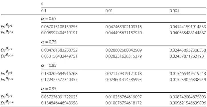
Table 1 Error estimates between the exact and regularized solutions forτ= 1.6, α∈ {0.65, 0.75, 0.85, 0.95}

0.1 0.01 0.001

α= 0.65

Errβpri _{0.067015108159255} _{0.047468902109316} _{0.041441591914833}

Errβpos _{0.098997404519191} _{0.044495631182970} _{0.040535488144887}

α= 0.75

Errβpri _{0.084761583230752} _{0.028602688042509} _{0.024458932308338}

Errβpos _{0.053156432449751} _{0.028231628315379} _{0.024378712621981}

α= 0.85

Errβpri _{0.130209694916768} _{0.021179319121018} _{0.015465349519243}

Errβpos _{0.122475577340357} _{0.024601414585993} _{0.015239026338959}

α= 0.95

Errβpri _{0.037276991722023} _{0.010256764619097} _{0.008742004875893}

Errβpos _{0.134846446943958} _{0.010076794618172} _{0.009621545639896}

Table 2 Error estimates between the exact and regularized solutions forτ= 1.7, α∈ {0.65, 0.75, 0.85, 0.95}

0.1 0.01 0.001

α= 0.65

Errβpri _{0.111131774567399} _{0.047840847429863} _{0.040796403046666}

Errβpos _{0.104219494973211} _{0.047373969253811} _{0.040704667266564}

α= 0.75

Errβpri _{0.042292184968334} _{0.032976631468816} _{0.025075858532616}

Errβpos _{0.118817648652812} _{0.028123860184860} _{0.024430674882777}

α= 0.85

Errβpri _{0.130527372052525} _{0.022400766773086} _{0.014919116713563}

Errβpos _{0.082465125249822} _{0.020184320450563} _{0.014652593632991}

α= 0.95

Errβpri _{0.045333767253358} _{0.011699213808191} _{0.008763429831879}

Errβpos _{0.044277712631869} _{0.008651113194266} _{0.008905712655202}

Step 3.Error estimate between the exact and regularized solutions:

E=

!Nx

i=0|f

β(xi) –f(xi)|2_L2_(0,1) !Nx

i=0|f(xi)|2L2_(0,1)

. (4.9)

The numerical results are summarized in Tables1,2,3.

Table1show the relative error estimates between the exact solution and its regularized solution, both a priori and a posteriori, atτ = 1.6 withα= 0.65,α= 0.75,α= 0.85, and

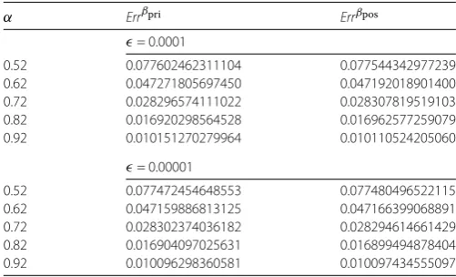
α= 0.95. Table2show the relative error estimates between the exact solution and its reg-ularized solution, both a priori and a posteriori atτ= 1.7 withα= 0.65,α= 0.75,α= 0.85, andα= 0.95. In Tables1and2, we calculate with values of= 10–1, 10–2 and= 10–3. In Table3, with two values= 10–4_and_{= 10}–5_,_τ _{= 1.8, we choose}_α_{= 0.52,}_α_{= 0.62,}

(19)

Table 3 Error estimates between the exact and regularized solutions forτ= 1.8, α∈ {0.52, 0.62, 0.72, 0.82, 0.92}

α Errβpri _Errβpos

= 0.0001

0.52 0.077602462311104 0.077544342977239

0.62 0.047271805697450 0.047192018901400

0.72 0.028296574111022 0.028307819519103

0.82 0.016920298564528 0.016962577259079

0.92 0.010151270279964 0.010110524205060

= 0.00001

0.52 0.077472454648553 0.077480496522115

0.62 0.047159886813125 0.047166399068891

0.72 0.028302374036182 0.028294614661429

0.82 0.016904097025631 0.016899494878404

0.92 0.010096298360581 0.010097434555097

rule method converges to the exact solution faster than the prior parameter choice rule method. We also see that our proposed regularized methods have very good convergence rates to the exact solution astends to 0.

5 Concluding remarks

In this work, we have studied the inverse source problem for the Rayleigh–Stokes equa-tion in a second-grade generalized ﬂow. We introduce a Tikhonov regularized method to establish an approximate solution. Then we prove an upper bound on the rate of conver-gence of the mean integrated squared error under some a priori condition of the sought solution. In the future work, we will try to study a numerical method for solving the ill-posedness of our inverse source problem.

Acknowledgements

Many thanks to Professor Nguyen Huy Tuan for discussing and helping to develop this paper.

Funding

Not applicable.

Availability of data and materials

Not applicable.

Competing interests

The authors declare that they have no competing interests.

Authors’ contributions

The authors declare that the study was realized in collaboration with the same responsibility. All authors contributed equally to the writing of this paper. All authors read and approved the ﬁnal manuscript.

Author details

1_{Faculty of Natural Sciences, Thu Dau Mot University, Thu Dau Mot, Vietnam.}2_{Department of Mathematics, School of}

Advanced Sciences, Vellore Institute of Technology, Vellore, India.3_{Institute of Computational Science and Technology,}

Ho Chi Minh City, Vietnam.4_{Institute of Research and Development, Duy Tan University, Da Nang 550000, Vietnam.} 5_{Applied Analysis Research Group, Faculty of Mathematics and Statistics, Ton Duc Thang University, Ho Chi Minh City,}

Vietnam.

Publisher’s Note

Springer Nature remains neutral with regard to jurisdictional claims in published maps and institutional aﬃliations.

Received: 11 March 2019 Accepted: 25 July 2019 References

(20)

2. Podlubny, I.: Fractional Diﬀerential Equations. Mathematics in Science and Engineering, vol. 198. Academic Press, San Diego (1990)

3. Shen, F., Tan, W., Zhao, Y., Masuoka, T.: The Rayleigh–Stokes problem for a heated generalized second grade ﬂuid with fractional derivative model. Nonlinear Anal., Real World Appl.7(5), 1072–1080 (2006)

4. Dehghan, M.: A computational study of the one-dimensional parabolic equation subject to nonclassical boundary speciﬁcations. Numer. Methods Partial Diﬀer. Equ.22(1), 220–257 (2006)

5. Dehghan, M.: The one-dimensional heat equation subject to a boundary integral speciﬁcation. Chaos Solitons Fractals32(2), 661–675 (2007)

6. Dehghan, M., Abbaszadeh, M.: A ﬁnite element method for the numerical solution of Rayleigh–Stokes problem for a heated generalized second grade ﬂuid with fractional derivatives. Eng. Comput.33, 587–605 (2017)

7. Mehrdad, L., Dehghan, M.: The use of Chebyshev cardinal functions for the solution of a partial diﬀerential equation with an unknown time-dependent coeﬃcient subject to an extra measurement. J. Comput. Appl. Math.235(3), 669–678 (2010)

8. Zaky, A.M.: An improved tau method for the multi-dimensional fractional Rayleigh–Stokes problem for a heated generalized second grade ﬂuid. Comput. Math. Appl.75(7), 2243–2258 (2018)

9. Singh, J., Secer, A., Swroop, R., Kumar, D.: A reliable analytical approach for a fractional model of advection-dispersion equation. Nonlinear Eng.8, 107–116 (2019)

10. Meng, R., Yin, D., Drapaca, C.S.: Variable-order fractional description of compression deformation of amorphous glassy polymers. Comput. Mech. (2019).https://doi.org/10.1007/s00466-018-1663-9

11. Kirane, M., Malik, A.S., Gwaiz, M.A.: An inverse source problem for a two dimensional time fractional diﬀusion equation with nonlocal boundary conditions. Math. Methods Appl. Sci.36(9), 1056–1069 (2013)

12. Tatar, S., Ulusoy, S.: An inverse source problem for a one-dimensional space–time fractional diﬀusion equation. Appl. Anal.94(11), 2233–2244 (2015)

13. Nguyen, H.L., Nguyen, H.T., Kirane, M., Duong, D.X.T.: Identifying initial condition of the Rayleigh–Stokes problem with random noise. Math. Methods Appl. Sci.42, 1561–1571 (2019)

14. Hajipour, M., Jajarmi, A., Baleanu, D., Sun, H.: On an accurate discretization of a variable-order fractional reaction–diﬀusion equation. Commun. Nonlinear Sci. Numer. Simul.69, 119–133 (2019)

15. Baleanu, D., Jajarmi, A., Asad, J.H.: Classical and fractional aspects of two coupled pendulums. Rom. Rep. Phys.71(1), 103 (2019)

16. Baleanu, D., Jajarmi, A., Hajipour, M.: On the nonlinear dynamical systems within the generalized fractional derivatives with Mittag-Leﬄer kernel. Nonlinear Dyn.94(1), 397–414 (2018)

17. Baleanu, D., Jajarmi, A., Bonyah, E., Hajipour, M.: New aspects of the poor nutrition in the life cycle within the fractional calculus. Adv. Diﬀer. Equ.2018, 230 (2018).https://doi.org/10.1186/s13662-018-1684-x

18. Kumar, D., Singh, J., Baleanu, D.: Analysis of a fractional model of Ambartsumian equation. Eur. Phys. J. Plus133, 259 (2018)

19. Cavalier, L.: Nonparametric statistical inverse problems. Inverse Probl.24(3), 034004 (2008)

20. Mai, A.P.N.T.: A statistical minimax approach to the Hausdorﬀ moment problem. Inverse Probl.24(4), 045018 (2008) 21. Mair, A.B., Ruymgaart, H.F.: Statistical inverse estimation in Hilbert scales. SIAM J. Appl. Math.56(5), 1424–1444 (1996) 22. Bazhlekova, E., Jin, B., Lazarov, R., Zhou, Z.: An analysis of the Rayleigh–Stokes problem for a generalized second-grade

ﬂuid. Numer. Math.131, 1–31 (2015)