R E S E A R C H
Open Access
Qualitative analysis of a harvested
predator-prey system with Holling-type III
functional response incorporating a prey
refuge
Jinghai Wang
*and Liqin Pan
*Correspondence: [email protected]
College of Mathematics and Computer Science, Fuzhou University, Fuzhou, Fujian 350002, People’s Republic of China
Abstract
A predator-prey model with simplified Holling type III response function
incorporating a prey refuge under sparse effect is considered. Through qualitative analysis of the model, at least two limit cycles exist around the positive equilibrium point with the result of focus value, the Hopf bifurcation under a prey refuge is obtained. We also show the influence of prey refuge. Numerical simulations are carried out to illustrate the feasibility of the obtained results and the dependence of the dynamic behavior on the prey refuge. Through the results of computer
simulation, it is further shown that under certain conditions the model has three limit cycles surrounding the positive equilibrium point.
Keywords: limit cycles; Holling type III; prey refuge; predator-prey model
1 Introduction
The dynamical relationship between predators and their preys is one of the dominant subjects in ecology and mathematical ecology due to its universal importance, see [–]. Some of the empirical and theoretical work have investigated the effect of prey refuges, the refuges used by prey have a stabilizing effect on the considered interactions, and prey extinction can be prevented by the addition of refuges [–].
Huanget al.[] studied the stability analysis of a prey-predator model with Holling type III response function incorporating a prey refuge:
⎧ ⎨ ⎩
dx
dt=ax–bx–
αxy
β+x, dy
dt = –cy+ kαxy
β+x.
(.)
Motivated by the study of Huanget al.[] and Ji and Wu [], we consider the following predator-prey model with Holling type III response function incorporating a prey refuge under sparse effect:
⎧ ⎨ ⎩
dx dt=rx
( –x k) –
(–m)xy a+(–m)x, dy
dt =y[–d+
u(–m)x a+(–m)x],
(.)
wherex(t) is the population density of the prey andy(t) is the population density of the predator at timet;r> represents the intrinsic growth rate of the prey;kis the carrying capacity of the prey in the absence of predator and harvesting;mis a constant number of prey using refuges, which protectsmof prey from predation; the termx/(a+x) denotes
the functional response of the predator, which is known as Holling type III response func-tion;u> is the conversion factor denoting the number of newly born predators for each captured prey;d> is the death rate of the predator.
From the point of view of human needs, the exploitation of biological resources and the harvest of population are commonly practiced in fishery, forestry, and wildlife man-agement. Concerning the conservation for the long-term benefits of humanity, there is a wide range of interest in the use of bioeconomic modeling to gain insight into the scientific management of renewable resources.
The problem of predator-prey interactions under a prey refuge have been studied by some authors. For example, Hassel [] showed that adding a large refuge to a model, which exhibited divergent oscillations in the absence of a refuge, replaced the oscillatory behavior with a stable equilibrium. McNair [] obtained that a prey refuge with legitimate entry-exit dynamics was quite capable of amplifying rather than damping predator-prey oscilla-tions. McNair [] showed that several kinds of refuges could exert a locally destabilizing effect and create stable, large-amplitude oscillations which would damp out if no refuge was present. Even now, prey refuges are widely believed to prevent prey extinction and damp predator-prey oscillations. For example, Kar [] considered a Lotka-Volterra type predator-prey system incorporating a constant proportion of prey using refugesm, which protectsmof prey from predation, with Holling type II response function and Holling type III response function, respectively. Our results indicate that refuge had a stabilizing effect on prey-predator interactions and the dynamic behavior very much depends on the prey refuge parameterm, point that increasing the amount of refuge could increase prey densities and lead to population outbreaks.
This article is organized as follows. Basic properties such as the existence, stability, and instability of the equilibria of the model and the boundedness of the solutions of the sys-tem (.) with positive initial values are given in Section . In Section , sufficient condi-tions for the global stability of the unique positive equilibrium are obtained. Section is devoted to deriving the existence of limit cycle. In Section , we study the Hopf bifurcation of system (.). In Section , we analyze the influence of prey refuge and give numerical stimulations.
2 Basic properties of the model
LetR+
={(x,y)|x≥,y≥}. For practical biological meaning, we simply study system (.)
inR+
. The main aim of this article is to study the existence and non-existence of positive
equilibrium of (.) by the effects of a prey refuge, that is to say, the existence and non-existence of positive equilibrium of system (.) depend on the constantm∈[, ).
We make the following substitution for model (.)
Denoting new argumentτwithtagain, it gives
⎧ ⎨ ⎩
dx dt =x
{r( –x
k)[a+ ( –m)
x] – ( –m)y}, dy
dt =y[–da+ (u–d)( –m)x].
(.)
Solutions of system (.) are discussed as follows:
() Ifu≤d, system (.) possesses only two equilibrium points on the regionR+, they are the trivial solutionO(, ) and the semi-trivial solution in the absence of predatorP(k, ); () Ifu>d, system (.) admits three equilibrium points on the regionR+, they are the trivial solutionO(, ), the semi-trivial solution in the absence of predatorP(k, ) and the unique positive constant solutionP(x,y), where
x= –m
da
u–d, y=r
–
k( –m)
da u–d
ua
(u–d)( –m).
For the existence of positive constant solutionP(x,y), it is necessary to assume that
–k(–m)
da
u–d> , then we derive that ≤m< – k
da u–d.
It turns out that the non-constant positive solutions of (.) may exist for some ranges of the parameterm. From the first equation of system (.), it is easy to derive that
lim sup
t→+∞ x(t)≤k.
Lemma . The solution(x(t),y(t))of system (.) with the initial value x() > , y() >
is positive and bounded for all t≥. Proof We see that dxdt|x=k= –(–m)
ky
a+(–m)k < withy> , sox=kis a untangent line of
sys-tem (.). And the positive trajectory of syssys-tem (.) goes through from its right side to its left side when it meets the linex=k.
Construct Dulac functionw(x,y) =y+ux–l, computingw= along the trajectories of system (.)
dw dt =
dy dt+u
dx
dtx= –dy+urx
–x
k
=urx
–x
k
–d(l–ux).
If l> is large enough, we have dwdt < , where <x<k. So the line y+ux=l goes through from its upside to its downside in the region{(x,y)| <x<k, <y< +∞}. For sys-tem (.), constructing a Bendixson ringOABC includingP(x,y). DefineOA,AB,BC
as the lengths of linesL=y= ,L=x–k= ,L=y+ux–l, respectively. The boundary line of the Bendixson ringOABC’s isJ. So, the orbits of system (.) enter into the interior of the Bendixson ring when it meets the boundary lineJ.
If the initial valuepwhich is in the first quadrant is not in theOABC, we can construct a curveJp in the same way, denotingp∈Jp. Thus the positive trajectoryL+pwhich is pass
throughpgoes through into the interior ofJpat the end. Note that the pointP(x,y) is
the unique equilibrium point in the Bendixson ringOABC. Through the Limit collection theory, we know that the trajectoryL+
p goes through into the interior of the Bendixson
Lemma . () O(, )is a stable node point;
Proof The Jacobian matrix of system (.) is given by
J(x,y)
if ( –m)
is a center or a focus. The proof is completed.
From Lemma ., ifP= –rx[(–m)
where
D=
x, E= r A( –m)x
a+ x( –m)–ax+ ( –m)
x
k – ( –m) y ,
N=
x, F= r A( –m)x
x( –m)–a+ ( –m)
x k , L= r
Ax
–x
k , M= r Akx
, G=(u–d)y
Ax
,
H=(u–d)
Ax
, I=u–d
Ax .
It is obvious thatD= NandHD= I. Then we make use of the method Poincare to calculate the focus value.
Construct a form progressionF(x,y) =x+y+∞k=Fk(x,y), whereFk(x,y) is thekth
homogeneous multinomials withxandy. Considering dF
dt|(.)=
∂F
∂t · ˆP(x,y) +
∂F
∂tQˆ(x,y) = , we can obtain that three multinomials
and four multinomials ofF(x,y) are equal to zero separately. Noting that xP(x,y) + yQ(x,y) = –H(x,y) we can obtain
H= Ex+ (G– D)xy+ Hxy.
LetF(x,y) =ax+axy+axy+ay, then we can obtain the following form:
y∂F
∂x –x
∂F
∂y =y
ax+ axy+ay–xax+ axy+ ay
= –ax+ (a– a)xy+ (a– a)xy+ay.
Fromy∂F
∂x –x
∂F
∂y =H, we can derive that
–ax+ (a– a)xy+ (a– a)xy+ay= Ex+ (G– D)xy+ Hxy.
Through the comparison method of correlates, we can obtain that
⎧ ⎪ ⎪ ⎪ ⎪ ⎪ ⎨ ⎪ ⎪ ⎪ ⎪ ⎪ ⎩
a=G– D,
a= –E, a= ,
a= –H+E,
thenF(x,y) =G– Dx– Exy–H+E yand
–H= xP+ yQ+
∂F
∂x ·P+
∂F
∂y ·Q
= (EG+ D– G– F)x+ (HG+ EG– I– DE)xy
Letx=rcosθ,y=rsinθ, then we can derive that
C=
H(cosθ,sinθ)dθ=
(G+ F+I+ DE– EG– D–HG).
Hence, then pointO(, ) of system (.) is an unstable fine focus with order one when
C> . But considering the time changedτ= –A dt,P(x,y) is a stable fine focus with
order one. AndP(x,y) is an unstable fine focus with order one whenC< . IfC= , namely G+ F+I+ DE– EG– D–HG= , we denote
F(x,y) =bx+bxy+bxy+bxy+by.
By substitutingF(x,y) =bx+bxy+bxy+bxy+byintoy∂∂Fx–x
∂F
∂y =H, by–bx+ (b– b)xy+ (b– b)xy+ (b– b)xy
= (G+ F– EG– D)x+ (I+ DE– HG– EG)xy
+D– N– GD– E– EHxy–H+ EHxy.
Through the comparison method of correlates, we can obtain that
⎧ ⎪ ⎪ ⎪ ⎪ ⎪ ⎪ ⎪ ⎪ ⎨ ⎪ ⎪ ⎪ ⎪ ⎪ ⎪ ⎪ ⎪ ⎩
b=D–N–GD–E–EH–H,
b= EG+ D– G– F=(I+ DE– HG– EG),
b= –H– EH,
b= ,
b= ,
then we have
F(x,y) =
D
–
N– GD–E
–
EH– H
x
+ (EG+ D– G– F)xy–H+ EHxy.
Also
–H= xP+ yQ+P
∂F
∂x +Q
∂F
∂y +P
∂F
∂x +Q
∂F
∂y
=–L– GF+ DF– DE+ NE+ GDE+ E+ EH+ EHx
+GN– DN+ EF+ EI+ D– GD– ED– EHD– HD
– EG– DE+ GE+ GH+ EGH– DH+ GH+ FHxy
+–EN+ EGD+ D– GD– FD+ EH+ EH
NotingF(x,y) =dx+dxy+dxy+dxy+dxy+dyinto y∂F
∂x –x
∂F
∂y =H,
through the comparison method of correlates, we can obtain that
⎧
we can derive that
C=
Hence pointO(, ) of system (.) is an unstable fine focus with second-order when
C> . But considering the time changedτ= –A dt, we know thatP(x,y) is a stable fine focus with second-order. AndP(x,y) is an unstable fine focus with second-order when
C< . The proof is completed.
Remark IfC= holds,P(x,y) is possible a fine focus with third-order.
3 Global stability of the unique positive equilibrium Theorem . Suppose that –√a
k ≤m< holds and there is no close orbit around system (.) in the first quadrant. Assume that:
Then the equilibrium P(k, )of system (.) is globally asymptotically stable on the first quadrant, if (H) holds. And the positive equilibrium P(x,y)of system (.) is globally asymptotically stable, if one of (H) and (H) holds.
Proof By Lemmas . and ., the solution (x(t),y(t)) of system (.) with the initial values
x() > ,y() > is unanimous bounded for allt≥ and the pointP(x,y) is globally
asymptotically stable, we should proof that the system (.) is not exist limit cycle if –√
a
4 Existence of limit cycle
Theorem . Suppose that≤m< –u+kdd(ua–d). Then system (.) exists at least one limit cycle in the first quadrant.
Proof In the proof of Lemma ., we can obtain the boundary lineJof the Bendixson ring
B={(x,y)| <x<k, <y<l–ux}. LetJbe the outer boundary of system (.). Due to the Lemma ., we know that there exists an unique unstable singular pointP(x,y) in the Bendixson ringB. By Poincare-Bendixson theorem, system (.) exists at least one limit cycle in the first quadrant. This completes the proof.
5 Hopf bifurcation
By the study of Louet al.[] and the Lemma . we have the following theorem:
Theorem . () If C> and < –u+dd·k
da
u–d–mhold, then system (.) exists a limit cycle around the small neighborhood of P(x,y). Further if the limit cycle is unique, then it is stable.
() If C< , <δ, <δ<δand <C<δ,–δ<P< hold, then system (.) exists at least two limit cycles around the small neighborhood of P(x,y).
By selecting the suitable values of the parameters, we can obtain these two limit cycle. () If C> , <δ, <δ<δand–δ<C< , <P<δhold, then system (.) exists at least two limit cycles around the small neighborhood of P(x,y). By selecting the suitable values of the parameters, we can obtain these two limit cycle.
6 The effect of prey refuge and harvesting efforts and examples
6.1 The influence of prey refuge on model (1.2)
By the variable transformationdt=a+ ( –m)xdτ, the positive equilibriumP
The above inequality shows thatxis a strictly increasing function with respect to the parametermand that the increasing of the prey refuge increases the density of the prey.
One could see thatyis also a continuous differential function of the parameterm. Sim-ple computation shows that
dy
We discuss (.) in the following two cases. Case : Assume that the inequality – k
allm> , thusyis a strictly decreasing function with respect to the parameterm. That
is, increasing the amount of prey refuge can decrease the density of the predator. In this case,yreaches the maximum valuer[ –k
thusyis a strictly increasing function of parameterm. That is, increase the amount of prey refuge can increase the density the predator. This analysis shows that increasing the amount of prey refuge can increase the density of the predator due to the predator still has enough food for predation withmbeing small.
6.2 Example and simulations
Figure 1 P2(x1,y1) is globally asymptotically stable withm= 0.49.
Figure 2 P2(x1,y1) is globally asymptotically stable withm= 0.43.
We known that –
√
a
k <m< – k
da
u–d, if we takem= . andm= . separately. By
Theorem ., system (.) admits a globally asymptotically stable equilibriumP(x,y) in the regionR+, which is shown in Figures and .
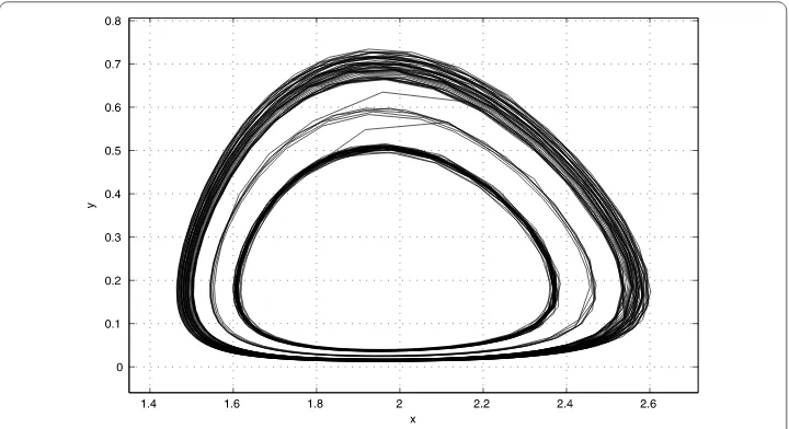
If we takem= . andm= . separately, by Theorem ., system (.) admits one and two limit cycles surrounding equilibriumP(x,y), which is shown in Figures and .
Example Letr= .,k= ,a=,d= ,u= in the system (.). By simple compu-tation, we have
–
√
a k = –
√
Figure 3 There is a stable limit cycle surroundingP2(x1,y1) withm= 0.134.
Figure 4 There are two limit cycles surroundingP2(x1,y1) withm= 0.113.
–
k
da u–d= –
√
= ., –u+ d
d ·
k
da u–d= –
√
= ..
If we takem= ., by Theorem ., system (.) admits three limit cycles surrounding equilibriumP(x,y), which is shown in Figure .
Figure 5 There are three limit cycles surroundingP2(x1,y1) withm= 0.065.
their equilibrium values, respectively, which means that if we change the value ofm, it is possible to prevent the cyclic behavior of the predator-prey system and to drive it to a required stable state.
7 Conclusion
This article considers a predator-prey model with Holling type III response function in-corporating a prey refuge under sparse effect. We give the complete qualitative analysis of the instability and global stability properties of the equilibria and the existence of limit cycles for the model. Our results, examples, and simulations indicate that dynamic behav-ior of the model very much depends on the prey refuge parametermand increasing the amount of refuge could increase prey densities and lead to population outbreaks.
Competing interests
The authors declare that they have no competing interests.
Authors’ contributions
All authors contributed equally and significantly in writing this paper. All authors read and approved the final manuscript.
Received: 26 May 2012 Accepted: 21 June 2012 Published: 2 July 2012
References
1. Holling, CS: Some characteristics of simple 240 types of predation and parasitism. Can. Entomol.91, 385-398 (1959) 2. Hassell, MP: The Dynamics of Arthropod Predator-Prey Systems. Princeton University Press, Princeton (1978) 3. Hoy, MA: Almonds (California). In: Helle, W, Sabelis, MW (eds.) Spider Mites: Their Biology, Natural Enemies and
Control. World Crop Pests, vol. 1B. Elsevier, Amsterdam (1985)
4. Sih, A: Prey refuges and predator-prey stability. Theor. Popul. Biol.31, 1-12 (1987)
5. Krivan, V: Effects of optimal antipredator behavior of prey on predator-prey dynamics: the role of refuges. Theor. Popul. Biol.53, 131-142 (1998)
6. Kar, TK: Stability analysis of a prey-predator model incorporating a prey refuge. Commun. Nonlinear Sci. Numer. Simul.10, 681-691 (2005)
7. Ko, W, Ryu, K: Qualitative analysis of a predator-prey model with Holling type II functional response incorporating a prey refuge. J. Differ. Equ.231, 534-550 (2006)
8. Collings, JB: Bifurcation and stability analysis of a temperature-dependent mite predator-prey interaction model incorporating a prey refuge. Bull. Math. Biol.57, 63-76 (1995)
9. Huang, Y, Chen, F, Zhong, L: Stability analysis of a prey-predator model with Holling type III response function incorporating a prey refuge. Appl. Math. Comput.182, 672-683 (2006)
11. McNair, JN: Stability effects of prey refuges with entry-exit dynamics. J. Theor. Biol.125, 449-464 (1987)
12. McNair, JN: The effects of refuges on predator-prey interactions: a reconsideration. Theor. Popul. Biol.29, 38-63 (1986) 13. Zhang, ZF, Ding, TR, Huang, WZ, Dong, ZX: Qualitative Theory of Differential Equations, 1st edn. Science Publishing
Company, Beijing (1985)
14. Lou, DJ, Zhxng, X, Dong, ZX: Qualitative and Branch Theory of the Dynamic System. Science Publishing Company, Beijing (1999)
doi:10.1186/1687-1847-2012-96