Study of pulsatile pressure driven electroosmotic flows through an elliptic cylindrical microchannel with the Navier slip condition

R E S E A R C H

Open Access

Study of pulsatile pressure-driven

electroosmotic flows through an elliptic

cylindrical microchannel with the Navier

slip condition

Pearanat Chuchard

_{, Somsak Orankitjaroen}

_{and Benchawan Wiwatanapataphee}

*_{Correspondence:}

[email protected]

1_{Department of Mathematics,}

Faculty of Science, Mahidol University, Rama VI Road, Bangkok, 10400, Thailand

2_{The Centre of Excellence in}

Mathematics, Si Ayutthaya Road, Bangkok 10400, Thailand Full list of author information is available at the end of the article

Abstract

This paper aims to study an unsteady electric field-driven and pulsatile

pressure-driven flow of a Newtonian fluid in an elliptic cylindrical microchannel with Navier boundary wall slip. The governing equations of the slip flow and distributions of electric potential and charge densities are the modified Navier-Stokes equations, the Poisson equation and the Nernst-Planck equations, respectively. Analytical and numerical analyses based on the Mathieu and modified Mathieu equations are performed to investigate the interplaying effects of pulsatile pressure gradients and the slip lengths on the electroosmotic flow.

Keywords: microchannel flow; elliptic cross-section; Navier-Stokes equations; pulsatile pressure gradient; elctroosmosis; electric potential

1 Introduction

Over the past decades, a fluid flow manipulation under a very small scale known as mi-crofluidics has become an active field of scientific research due to the emergence of their several applications, for example, lab-on-the-chips, computer chips, medical diagnostic devices, and drug delivery systems [–]. Taking the advantage of a small scale system, a microfluidic application not only reduces the requirement for the samples, but also in-creases the efficiency and speed of the reaction. As a consequence, the microflow char-acteristics have been widely studied in both experimental and analytical ways in order to develop various system controls and device designs [–]. One particular technique to precisely manipulate a flow in a microscale is the use of a pressure force combined with the well-known electrokinetic force, namely, electroosmosis. Electroosmosis phenomenon re-lies on the formation of the electrical double layer (EDL) generated by two parallel layers of charged ions: the first layer, the layer of ions on the inner wall surface due to the chem-ical reaction between the fluid and the channel wall; the second layer, the layer of counter ions in the fluid attracted to the first layer by the Coulomb force. The movement of the ions in the second layer, induced by the application of an external electric field, will lead to the motion of the entire fluid caused by the drag force [].

Fluid flow problems have been carried out traditionally under the no-slip boundary con-dition [–], which dictates that the velocity, relative to the wall channel, of the fluid ad-jacent to the wall is zero. However, in microfluidics, the appearance of the fluid slip at the wall interface has been widely reported, and its influence has been investigated [–]. For this reason, the velocity slip condition turns into an important factor to achieve the realistic microflow behavior.

In the literature, an analytic solution of an electroosmotic flow in microchannels has been studied under a constant pressure gradient. Goswami and Chakraborty [] inves-tigated the semi-analytic solution of a steady electroosmotic flow with the interfacial slip condition in microchannels of various complex cross-sectional shapes under the constant pressure gradient assumption. Naet al. [], Chinyoka and Makinde [], and Reshadet al. [] found the analytic solution of transient electroosmotic and pressure-driven flows with a constant pressure gradient through a microannulus, a slip microchannel, and rect-angular microchannels, respectively. However, some microfluidic systems are driven by a pulsatile pressure gradient due to the nature of some systems such as blood flow or the integrated micropump of displacement type. Moreover, a report of Bandopadhyay and Chakraborty [] on the investigation of electroosmotic flow in a slip microchannel shows that the overestimation result can be obtained under the avoidance of a pulsating pressure gradient. As a result, a microfluidic investigation combined with a pulsating pressure gra-dient is a key to keeping the problem suitable in many situations. Recently, the solution of combined pulsating pressure gradient and electroosmotic flow was found by Chakraborty

et al. [], but the pressure gradient was simplified to just a sinusoidal function.

Due to the fact that the geometry in many microfluidic devices and some systems such as a blood vessel is of a circular or elliptic cross-section, the use of elliptic geometry takes an advantage of embodying the solution for circular geometry and making the problem tractable for any eccentricity.

According to the aforementioned arguments, we here derive the solution of com-bined pulsatile pressure-driven and electroosmotic flow through an elliptic cylindrical microchannel under the Navier slip condition to describe the flow behavior in a more realistic situation than the previous works. The pressure gradient term in Navier-Stokes equations is precisely expanded by the Fourier series. Moreover, an influence of a pulsatile pressure gradient, the number of the Fourier expansion terms for the pressure gradient, and a slip length are investigated on the volumetric flow rate which plays a more important role in the flow control in microfluidic devices compared to the velocity profile.

2 Preliminaries

In this section, we introduce the elliptic cylindrical coordinates, the Mathieu and modified Mathieu functions which are used throughout this paper.

2.1 Elliptic cylindrical coordinate system

Considering an elliptic cylindrical geometry having two foci on x-axis atx=±cof the Cartesian coordinate system (x,y,z), we define the elliptic cylindrical coordinates (ξ,η,z) by

where ≤ξ <∞, ≤η< π, and –∞<z<∞. The coordinatesξ andηrespectively correspond to the confocal elliptic cylinder and the asymptotic angle of the confocal hy-perbolic cylinder with the identities

x c_cosh_ξ +

y

c_sinh_ξ =  and

x c_cos_η–

y c_sin_η= .

The scale factors are

hξ=hη=c

coshξ–cos_{η and h}

z= ,

and the Laplacian is

∇₌ 

c_(cosh_ξ–cos_η)

∂ ∂ξ+

∂ ∂η

+ ∂



∂z.

2.2 Mathieu functions

The solutions of the -dimensional wave equation in the elliptical coordinates,



c_(cosh_ξ–cos_η)

∂W

∂ξ +

∂W

∂η

+kW= , ()

were introduced by the French mathematician, Émile Léonard Mathieu, in  as the eigensolutions of the Mathieu differential equations to determine the motion of an elliptic stretched membrane []. The method splits equation () into two ordinary differential equations with the separation constantaas follows:

d_G

dη + (a– qcosη)G= , ()

d_F

dξ – (a– qcoshξ)F= , ()

whereq=k_c_{/ > . Equations () and () are respectively named the Mathieu and}

mod-ified Mathieu equations, and their solutions corresponding to special values of the sep-aration constant (characteristic numbers) are called the Mathieu and modified Mathieu functions. These characteristic numbers are the functions ofq. Hence, the solutions of equation (), in an elliptic geometry, can be written as a linear combination of the peri-odic Mathieu functions ofηand the modified Mathieu functions ofξ:

W(ξ,η) = ∞

m=

CmCem(ξ,q)cem(η,q) +CmFem(ξ,q)cem(η,q)

+SmSem(ξ,q)sem(η,q) +SmGem(ξ,q)sem(η,q)

, ()

wherecem(η,q),sem(η,q) are the periodic Mathieu functions;Cem(η,q),Sem(η,q) are the

3 Mathematical modeling

In this section, we construct the fundamental equation of the problem. The govern-ing equations of a transient electroosmotic flow for an incompressible Newtonian fluid through an elliptical tube, with thez-axis being the channel-length direction, are the con-tinuity equation and the incompressible Navier-Stokes equations as given below:

∇ ·v= , ()

pressure, andμis the viscosity. The electrokinetic body force Fekis defined by Fek=ρeE,

where E is the external electric field andρeis the ionic charge density given by the Poisson

equation

∇_{ψ(ξ,η) = –}ρe

ε, ()

whereεis the permittivity of the fluid andψ is the potential inside the channel. In this study, we focus on a fully developed flow along thez-axial direction,i.e., v = (, ,vz), ∇p= (, ,∂p/∂z), E = (, ,E). Then the continuity equation () now becomes∂vz/∂z= ,

which gives rise tovz=u(ξ,η,t), and the incompressible Navier-Stokes equations () can

be reduced to the form

∇

As mentioned before, in this study, we consider a time periodic function of the pressure gradient driving the flow. To be precise,∂p/∂zis time periodic and can be expressed by

∂p

andωis the frequency. As equation () is linear, we can use the superposition principle for the solution,i.e., ifUnis a solution of equation () for∂p/∂z=cnexp(inωt), then the

complete solution of equation () for∂p/∂z=Re(_n∞_=cnexp(inωt)) isU=

∞

n=Re(Un).

For the electrical double layer field acting only in the direction perpendicular to the boundary, the boundary conditions for the potential distributionψare as follows: (i)ψis constant on the boundary and (ii)∂ψ/∂n=  at the center of the channel. Consider that fluid flow and the potential distribution are symmetric aboutx- andy-axes, the boundary conditions in elliptic cylindrical coordinates are given by

∂u

with the Navier slip condition of a non-movement channel

u(ξ,η,t) +

l

ccoshξ–cosη

∂u

∂ξ(ξ,η,t) = , (d)

and the constant zeta potentialζ at the wall

ψ(ξ,η) =ζ, (e)

wherelis the slip length,ξ=ln(( +

√

 –e¯₎¯_e–_{) is the boundary interface, ande¯is the}

eccentricity of the ellipse.

4 Solution of the boundary value problem

In this section, we construct the solution of transient combined pulsatile pressure-driven and electroosmotic flow for an incompressible Newtonian fluid through an elliptical tube. Hereafter, the symbol denotes the differentiation with respect toξ. To determine the velocityu(ξ,η,t), we solve

For constant pressure (n= ), equation () becomes

∂f

The non-homogeneous equation () can be solved by the eigenfunction expansion with the boundary conditions (a)-(c), and thus the solutionfis in the form

Equation () is now in the form of the -dimensional wave equation in elliptic coordi-nates, and hence, the solutionsWnare in the form of the Mathieu and modified Mathieu

equations as we mention in Section . forq= –isn= –inωρc{μ}–. In this study, we

as-sume thatUis symmetrical aboutx- andy-axes. Since the symmetry is governed by the function ofηand onlycem(η,q) are symmetrical about the both axes, the solutions in the

form of equation () can be simplified to

Wn(ξ,η) =

to satisfy the boundary condition (c). Hence, the solutionsWncan be reduced to

Wn(ξ,η) =

∞

m=

Bn_mCem(ξ, –isn)cem(η, –isn).

From the superposition principle, the flow velocityuis in the form

u(ξ,η) = εE

boundary condition (d) using the value ofψ in equation (e). By equating the terms having the same exponential, we then have

 =εE

Mathieu functions, respectively:

Forl> , letkbe a non-negative integer. Multiplying equations () and () bycos(kη) andcek(η, –isn) respectively and integrating from  to πwith respect toη, we then have

the following system of equations:

∞

Equations () represent the infinite system of linear equations which can be used to com-pute the approximate values ofAmandBnmby reducing it to a system with finite terms

ofn,mandk,i.e.,n= , , , . . . ,N;m= , ,  . . . ,Mandk= , , , . . . ,Kfor suitable fixed positive numbersN,M, andK.

The solutionsUn, until now, contain the unknown potentialψ. In order to findψ(ξ,η),

we assume that the influence of the convection is negligible and the electrolyte is symmet-ric. Hence, the ionic charge density can be expressed using the Boltzmann distribution of the number density of positive and negative ions as

pe=ezν(n+–n–) =ezνnsinh

wheren±is the number density of the positive and negative ions,εis the permittivity of the fluid,nis the ionic concentration at the bulk,eis the elementary charge of a proton,

Combining equations () and (), we calculateψ through the Poisson-Boltzmann

equa-In the case of a low value of zeta potential, the Poisson-Boltzmann equation () is reduced to the Debye-Hückel approximation

the potentialψ in equation () can be obtained in a similar way. Using the boundary conditions (a)-(c) and (e), we then have

ψ(ξ,η) =

As the fluid velocity is now known, the volumetric flow rate can be calculated through the formula

According to this formula, the numerical results of volumetric flow rate will be presented in the next section.

5 Numerical results and discussions

In this section, we show some numerical results of velocity profile under the oscillating pressure gradient and the electrokinetic force through an elliptical cylindrical channel at various times during a wave cycle. The presented results are achieved using the formula in equation () where the coefficientsAm,Bnmare defined by equation () for the no-slip

condition (l= ) and equation () with the appropriate numbersM=K=  for the slip condition (l> ). The solution in equation () is more general than the one in []; in other words, when the external electric field is zero and the pressure gradient does not oscillate (dp/dz=c), our solution reduces to

which is exactly the one presented in [].

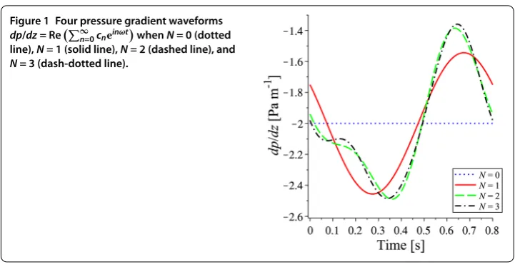
Figure 1 Four pressure gradient waveforms dp/dz= Re∞n=0cneinωt

whenN= 0 (dotted line),N= 1 (solid line),N= 2 (dashed line), and N= 3 (dash-dotted line).

slip lengthslare presented. Moreover, an influence of oscillating term in a pressure gra-dient expression on electroosmotic flows with various external electric fields are investi-gated.

In this section, we use the fluid properties as appeared in Li’s work []. The fluid is aqueous KCl solution (: electrolyte) with the properties prescribed in parameters as follows: ρ= .×_{kg m}_{; μ= .× }–_{kg m}–_s–_{; ε= .×}–_{C V}–_m–_;

ζ = .×–_{V; andκ= ×}_m–_{. The channel is the rigid tube of elliptic}

cross-section having the focus lengthc= μm and the eccentricitye¯= .. The waveform of pressure gradient as shown in Figure  is determined by setting the parametersc= –,

c= . + .i,c= –. + .i,c= –. + .i, andω= π(.)–. Since the

elec-troosmotic force in this study is considered to be positive, the negative pressure gradient force will reinforce the electroosmotic flow.

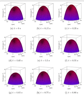
As the velocityuin equation () does not depend onz, the velocity profiles of mixed electroosmotic pressure-driven flow through the elliptical cylindrical channel are pro-jected to the elliptic cross-section presented in Figure . The results are plotted using

N= ,l= μm, andE=  V m–_{at nine different timest= , ., ., ., ., .,}

., ., and . s. The result shows the relation of flow to an oscillatory pressure gradi-ent. The graph of velocity represents the forward flow with speed of .μm s–as a result of the positive electrokinetic force combined with the positive pressure force (negative pressure gradient). For .≤t≤. s, the amplitude of the (negative) pressure gradient increases as time increases. This results in the increased pressure force, which causes an increase in the flow speed. Att= . s, as the (negative) pressure gradient decreases to the nadir (maximum amplitude), the forward speed reaches μm s–. For .≤t≤. s, the amplitude of the (negative) pressure gradient decreases as time increases. This means that the pressure force decreases. As a result, the velocity combined with the pressure force drops. Att= . s, the velocity reduces to μm s–_{because the (negative)}

pres-sure gradient increases to the peak (minimum amplitude). For .≤t≤. s, the velocity increases as the amplitude of pressure gradient increases. Att= . s, the end of pressure gradient wave, the velocity profile is similar to the one att=  s.

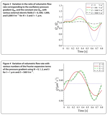
Figure  shows the variation in the ratio of volumetric flow rates corresponding to the oscillatory pressure gradientQppand the constant oneQcpwith various external electric

Figure 2 Velocity profiles with various timest= 0, 0.15, 0.35, 0.45, 0.5, 0.55, 0.65, 0.75, and 0.8 s for l= 1μm, andE= 500 V m–1.

and -term of the Fourier expansion for the pressure gradient (N=  andN= ) is used in the case ofQcpandQpp, respectively. It can be seen that the ratioQpp/Qcpis in a wave

form and its amplitude decreases with an increase of E from  to , V m–_{; when}

E= , V m–_{, the ratioQ}

pp/Qcptends to a constant at . This physically means that,

forE= , the flow is driven only by the pressure force. In this case, the result shows an ex-treme difference of the volumetric flow rate with and without considering the oscillating term of the pressure gradient. For ≤E≤, V m–_{, the flow is driven by both the}

pressure gradient and the electroosmotic force. In this case, the effect of the oscillating term still significantly affects the volumetric flow rate. ForE= , V m–_{, the}

electroos-motic force becomes dominant. In this case, there is a slight difference between the flow rates Qpp andQcp. As a consequence, the pressure gradient force is practically

Figure 3 Variation in the ratio of volumetric flow rate corresponding to the oscillatory pressure gradientQppand the constant oneQcpwith

various external electric fieldsE= 0, 500, 1,000, and 5,000 V m–1_{forN= 3 andl= 1μm.}

Figure 4 Variation of volumetric flow rate with various numbers of the Fourier expansion terms of the pressure gradient usingN= 0, 1, 2, and 3 forl= 1μm andE= 500 V m–1_.

in the microchannel of elliptic cross-section when the flow is evidently driven by both the pulsatile pressure gradient and the electrokinetic force.

Figure  shows the variation of volumetric flow rate corresponding to various numbers of the Fourier expansion terms of the pressure gradient usingN= , , , and  forl= μm andE=  V m–. It can be seen that the flow rate has a constant value of .μms– when N=  (constant pressure gradient). The reasons for this occurrence are that the interpolation using only the first term of the Fourier series for the pulsatile pressure gra-dient represents just the mean pressure gragra-dient, and the electroosmotic force is a con-stant. WhenN≥, our results, related to the oscillation of the pressure gradient, develop traveling wave of fluid flow. ForN= , the flow rate is in a sinusoidal form as a result of the sinusoidal interpolation of the pressure gradient. In the cases ofN=  and , the flow rates appear to be similar and much closer together, but different from the flow rate when

N= . This investigation indicates the significance of using the higher Fourier expansion term for pressure gradient to manipulate the flow rate. However, when a pressure gradient is approximated well enough, the numerical result of flow rate is precise and reliable.

Figure 5 Variation of volumetric flow rate with various slip lengthsl= 0, 1, 2, 3, 4, and 5μm for N= 3 andE= 500 V m–1_.

-terms Fourier expansion (N= ) of the pressure gradient andE=  V m–_{. The}

re-sult shows that, for the particular value of the flow parameters used in this section, the volumetric flow rate with μm slip length increases compared with the no-slip flow rate. This result is consistent with the experiment in [] and the numerical result obtained from the analytical solution of a circular microchannel []. In fact, both claimed results imply that the velocity increases on the entire velocity profile when the slip condition is taken into consideration. A velocity increase will directly result in an increase in the flow rate. However, it can be seen that the flow rate ofl= μm is only % difference in value compared to the one of no-slip condition. It may be concluded that when the slip length is less than μm, the slip condition can be omitted to reduce the computational cost. Fig-ure  also shows that the flow rate gradually increases as the slip length increases. The flow rate increases to approximately %, %, %, and % higher whenl= , , , and μm, respectively. This result agrees well with the one obtained in [], which presents the ve-locity shift constantly upwards as the slip length increases. For the flow with higher slip length, the slip condition should be considered in the mathematical model to bring a more accurate result.

6 Conclusions

Competing interests

The authors declare that they have no competing interests.

Authors’ contributions

All authors read and approved the final manuscript.

Author details

1_{Department of Mathematics, Faculty of Science, Mahidol University, Rama VI Road, Bangkok, 10400, Thailand.}2_The

Centre of Excellence in Mathematics, Si Ayutthaya Road, Bangkok 10400, Thailand.3_{Department of Mathematics and}

Statistics, Faculty of Science and Engineering, Curtin University, Perth, WA, Australia.

Acknowledgements

This work is partially supported by Development and Promotion of Science and Technology Talents Project (DPST).

Publisher’s Note

Springer Nature remains neutral with regard to jurisdictional claims in published maps and institutional affiliations.

Received: 31 January 2017 Accepted: 17 May 2017 References

1. Gad-el-Hak, M: The fluid mechanics of microdevices - the Freeman scholar lecture. J. Fluids Eng.121(1), 5-33 (1999) 2. Beskok, A, Korniadakis, GE: Report: a model for flows in channels, pipes, and ducts at micro and nano scales.

Microscale Thermophys. Eng.3(1), 43-77 (1999)

3. Araki, T, Kim, MS, Suzuki, K: An experimental investigation of gaseous flow characteristics in microchannels. Microscale Thermophys. Eng.6(2), 117-130 (2002)

4. Saidi, F: Non-Newtonian flow in a thin film with boundary conditions of Coulomb’s type. Z. Angew. Math. Mech.

86(9), 702-721 (2006)

5. You, D, Moin, P: Effects of hydrophobic surfaces on the drag and lift of a circular cylinder. Phys. Fluids19(8), 081701 (2007)

6. Yang, J, Kwok, DY: Microfluid flow in circular microchannel with electrokinetic effects and Navier’s slip condition. Langmuir19(4), 1047-1053 (2003)

7. Duan, Z, Muzychka, YS: Slip flow in elliptic microchannels. Int. J. Therm. Sci.46, 1104-1111 (2007) 8. Duan, Z: Slip flow in doubly connected microchannels. Int. J. Therm. Sci.58, 45-51 (2012)

9. Lee, HB, Yeo, IW, Lee, KK: Water flow and slip on NAPL-wetted surfaces of a parallel-walled fracture. Geophys. Res. Lett.

34(19), L19401 (2007)

10. Goswami, P, Chakraborty, S: Semi-analytical solutions for electroosmotic flows with interfacial slip in microchannels of complex cross-sectional shapes. Microfluid. Nanofluid.11(3), 255-267 (2011)

11. Li, D: Electrokinetics in Microfluidics. Elsevier, Amsterdam (2004)

12. Goldstein, D, Handler, R, Sirovich, L: Modeling a no-slip flow boundary with an external force field. J. Comput. Phys.

105(2), 354-366 (1993)

13. Feng, ZG, Michaelides, EE: Robust treatment of no-slip boundary condition and velocity updating for the lattice-Boltzmann simulation of particulate flows. Comput. Fluids27(2), 370-381 (2009)

14. Bolintineanu, DS, Lechman, JB, Plimpton, SJ, Grest, GS: No-slip boundary conditions and forced flow in multiparticle collision dynamics. Phys. Rev. E, Stat. Nonlinear Soft Matter Phys.86(6), 066703 (2012)

15. Cohen, Y, Metzner, AB: Apparent slip flow of polymer solutions. J. Rheol.29(1), 67-102 (1985)

16. Tretheway, DC, Meinhart, CD: Apparent fluid slip at hydrophobic microchannel walls. Phys. Fluids14(3), 9-12 (2002) 17. Choi, CH, Westin, WJA, Breuer, KS: Apparent slip flows in hydrophilic and hydrophobic microchannels. Phys. Fluids

15(10), 2897-2902 (2003)

18. Na, R, Jian, Y, Chang, L, Su, J, Liu, Q: Transient electro-osmotic and pressure driven flows through a microannulus. Open J. Fluid Dyn.3(2), 50-56 (2013)

19. Chinyoka, T, Makinde, OD: Analysis of non-Newtonian flow with reacting species in a channel filled with a saturated porous medium. J. Pet. Sci. Eng.121, 1-8 (2014)

20. Reshadi, M, Saidi, MH, Firoozabadi, B, Saidi, MS: Electrokinetic and aspect ratio effects on secondary flow of viscoelastic fluids in rectangular microchannels. Microfluid. Nanofluid.20, 117 (2016)

21. Bandopadhyay, A, Chakraborty, S: Electrokinetically induced alterations in dynamic response of viscoelastic fluids in narrow confinements. Phys. Rev. E85, 056302 (2012)

22. Chakraborty, J, Ray, S, Chakraborty, S: Role of steaming potential on pulsating mass flow rate control in combined electroosmotic and pressure-driven microfluidic devices. Electrophoresis33, 419-425 (2012)

23. Mathieu, EL: Mémoire sur le mouvement vibratoire d’une membrane de forme elliptique. J. Math. Pures Appl.13, 137-203 (1868)

24. Mclachlan, NW: Theory and Application of Mathieu Functions. Clarendon, Oxford (1947)