Rational iterated function system for positive/monotonic shape preservation

R E S E A R C H

Open Access

Rational iterated function system for

positive/monotonic shape preservation

AKB Chand

_{, N Vijender}

_{and RP Agarwal}

*_{Correspondence: [email protected]} 1_{Department of Mathematics,} Indian Institute of Technology Madras, Chennai, 600036, India Full list of author information is available at the end of the article

Abstract

In this paper we consider the (inverse) problem of determining the iterated function system (IFS) which produces a shaped fractal interpolant. We develop a new type of rational IFS by using functions of the form Ei_Fi, whereEiare cubics andFiare

preassigned quadratics having 3-shape parameters. The fixed point of the developed rational cubic IFS is inC1, but its derivative varies from a piecewise differentiable function to a continuous nowhere differentiable function. An upper bound of the uniform error between the fixed point of a rational IFS and an original function

scaling factors and shape parameters in the rational IFS are formulated so that its fixed point preserves the positive/monotonic features of prescribed data. The presence of scaling factors provides additional freedom to the shape of the fractal interpolant over its classical counterpart in the modeling of discrete data.

1 Introduction

Setting a novel platform for the approximation of natural objects such as trees, clouds, feathers, leaves, flowers, landscapes, glaciers, galaxies, and torrents of water, Mandelbrot [] introduced the term fractal in the literature. Since fractals capture the non-linear struc-tures of various objects effectively, the fractal geometry has been successfully used in dif-ferent problems in applied sciences and engineering [–]. The iterated function system (IFS) was introduced by Hutchinson [] for the construction of various types of fractal sets, and popularized by Barnsley []. An IFS is a dynamical system consisting of a finite collection of continuous maps. Based on the IFS theory, Barnsley [] constructed a class of functions that are known as FIFs. The graph of a FIF is thefixed pointof an IFS. Also a FIF is thefixed pointof the Read-Bajraktarević operator on a suitable function space. Common features between a FIF and a piecewise polynomial interpolation are that they are geometrical in nature, and they can be computed rapidly, but the main difference is the fractal character,i.e., a FIF satisfies a functional relation related to the self-similarity on smaller scales. In the direction of smooth fractal curves, Barnsley and Harington [] initiated the construction of a restricted class of differentiable FIF orCk-FIF that interpo-lates the prescribed data if the values of(p),p= , , . . . ,k, at the initial end point of the interval are given, whereis the original function. This method is based on the recursive nature of an algorithm, and specifying the boundary conditions similar to the classical splines was found to be quite difficult to handle in this construction. The fractal splines with general boundary conditions have been studied recently [–] by restricting their IFSs parameters suitably.

The motivation of this work is the research on different types of splines by several au-thors; see, for instance, Schmidt and Heß [], Fritsch and Carlson [], Schumaker [], and Brodlie and Butt [], and references therein. The uniqueness of spline representation for a given data set turns out to be a disadvantage for shape modification problems. The use of rational functions with the shape parameters was introduced by Späth [] to pre-serve different geometric properties attached to a given set of data. Rational interpolants are often used in data visualization problems due to their excellent asymptotic proper-ties, capability to model complicated smooth structures, better interpolation properproper-ties, and excellent extrapolating powers. Gregory and Delbourgo [] introduced the rational cubic spline with one family of shape parameters, and this work inspired a large amount of research in shape-preserving rational spline interpolations, see [, ] and references therein.

In this paper, we introduce the rational cubic IFS with -shape parameters in each subin-terval of the interpolation domain such that its fixed point generalizes the corresponding classical rational cubic spline functions []. The developed rational cubic spline FIF is bounded, and is unique by fixed point theory for a given set of scaling factors and shape pa-rameters. Because of the recursive nature of FIF, the necessary conditions for monotonic-ity on the derivative values at knots alone may not ensure the monotonicmonotonic-ity of a rational cubic fractal interpolant for a given monotonic data. Based on the appropriate condition on the rational IFS parameters: (i) the scaling factors that depend only on given data, and (ii) the shape parameters that depend on both the interpolation data and scaling factors, we construct the shape-preserving rational cubic FIFs for a prescribed positive and/or monotonic data. By varying the scaling factors (within the shape-preserving interval) and shape parameters (according to the conditions derived in our theory), we can make the fixed point of a rational cubic IFS more pleasant and suitable for aesthetic requirements in a modeling problem. The proposed method is suitable for the shape-preserving inter-polation problems where a data set originates from an unknown function∈Cand its derivativeis a continuous nowhere differentiable function, for instance, the motion of single inverted pendulum in non-linear control theory [].

Comparison of the proposed rational cubic FIF over some existing schemes:

• When all the scaling factors are zero, the proposed rational cubic FIF reduces to the classical rational cubic interpolant [], see Remark , Section .

• To generate shape-preserving interpolants, our construction does not need additional knots in contrast to methods due to Schumaker [] and Brodlie and Butt [], which require additional knots for the shape-preserving interpolants.

• The classical interpolants [, ] are suitable only for monotonicity interpolation whereas the proposed rational cubic FIF is suitable for both monotonicity and positivity interpolation. Moreover, the rational quadratic interpolant [] is a special case of our rational cubic FIF for the particular choice of the scaling factors and shape parameters, see Remark , Section .

• Where monotonicity is concerned, our construction does not need an additional condition on derivatives at knots except for the necessary conditions. But the construction of Fritsch and Carlson [] needs some restrictions on derivatives at knots apart from the necessary conditions for the same problem.

• The derivatives of the shape-preserving interpolants [–, ] are piecewise smooth, whereas the derivative of our rational cubic FIF may be piecewise smooth to a non-differentiable function according to the choice of the scaling factors. Owing to this special feature, the proposed method is preferable over the classical

shape-preserving interpolants when the approximation is taken for data originating with an unknown function∈C_{having a shape with fractality in.}

This paper is organized as follows. In Section , the general constructions of fractal in-terpolants andCr_{-rational cubic FIFs based on IFSs are summarized. Section  is devoted}

to the construction of a suitable rational IFS so that its fixed point is the desired inter-polant that can be used for shape preservation. Then we deduce an upper bound of the uniform error bound between the original function and the rational cubic FIF. The fixed point of this rational IFS does not follow any shape constraints. The restrictions on the rational IFS parameters are deduced for a positivity shape in Section , and the results are illustrated with suitably chosen examples. In Section , the monotonicity problem is considered through the developed rational cubic IFS.

2 IFS for fractal functions

Letx<· · ·<xnbe a partition ofI= [x,xn]. Letfibe the value of original function atxi, i= , , . . . ,n. DenoteIi= [xi,xi+],C=I×D,Ci=Ii×D, and letDbe a compact sub-set

ofRsuch thatfi∈D, i= , , . . . ,n. LetLi(x) =aix+bi:I→Ii,i= , , . . . ,n– , be the

contractive homeomorphisms such that

Li(x) =xi, Li(xn) =xi+. ()

It is easy to verify that{I;Li(x),i= , , . . . ,n– }is a just touching hyperbolic IFS whose

unique fixed point is

I=

n–

i=

Li(I). ()

LetFi(x,f) =ξif +qi(x),|ξi|< ,i= , , . . . ,n– , be the continuous real-valued functions

onCsuch that

Fi(x,f) =fi, Fi(xn,fn) =fi+, ()

andqi:I→R,i= , , . . . ,n– , are the suitable continuous functions. Now define the

functionswi:C→Ci,∀i= , , . . . ,n– , aswi(x,f) = (Li(x),Fi(x,f)) for every (x,f)∈C.

ThenI≡ {C;wi(x,f),i= , , . . . ,n– }is called an IFS related to a given interpolation data

{(xi,fi),i= , , . . . ,n}. According to [], the IFSI has a unique fixed pointGwhich is the

graph of a continuous functionφ:I→R,φ(xi) =fi,i= , , . . . ,n. The functionφis called

a FIF generated by the IFSI, and it takes the form

φLi(x)

The existence of a spline FIF based on a polynomial IFS is given in []. We have extended this result to the rational IFS with -shape parameters in the following.

Theorem  Let{(xi,fi),i= , , . . . ,n}be a given data set,where diare the slope at xi,and d_i(k)(k= , . . . ,r)are the kth derivative values at xifor i= , , . . . ,n.Consider the rational IFSI∗≡ {I×D;wi(x,f) = (Li(x),Fi(x,f)),i= , , . . . ,n– },where Li(x) =aix+bisatisfies equation(),Dis a suitable compact sub-set ofR.Fi(x,f) =ari(ξif+qi(x)),

i,(x)

i,(x),i,(x)is a polynomial containingr+ arbitrary constants,andi,(x)is a non-vanishing quadratic

polynomial with-shape parameters in each subinterval defined on I, and|ξi| ≤κ < , i= , , . . . ,n– .Let F_i(k)(x,f) =a_ir–k(ξif+q(ik)(x)),where q

(k)

i (x)represents the kth derivative of qi(x)with respect to x.With the setting fi=di(),di=di(),i= , , . . . ,n,if

F_i(k)x,d(k)

=d(_ik), F_i(k)xn,d(nk)

=d_i(_+k), i= , , . . . ,n– ,k= , , . . . ,r, ()

then the fixed point of the rational IFSI∗is the graph of theCr-rational FIF.

Proof SupposeFr_={h∈Cr_[x

,xn]|h(x) =fandh(xn) =fn}. Now (Fr,dr) is a complete

metric space, wheredr_{is the metric onF}r_{induced by theC}r_{-norm onC}r_[x

,xn]. Define

the Read-Bajraktarević operatorUonFras

Uh(x) =ar_iξih

L–_i (x)+qi

L–_i (x), x∈Ii,i= , , . . . ,n– . ()

Sinceai=x_xi+_n––_xx_i< , the conditions|ξi| ≤κ<  and () imply thatUis a contractive

op-erator on (Fr,dr). The fixed pointψofUis a fractal function that satisfies the functional equation:

ψLi(x)

=ar_iξiψ(x) +qi(x)

, x∈I,i= , , . . . ,n– . ()

Sinceψ∈Cr[x,xn],ψ(k)satisfies

ψ(k)Li(x)

=ar_i–kξiψ(k)(x) +q(ik)(x)

, x∈I,i= , , . . . ,n– ,k= , , . . . ,r. ()

Using equation () in equation (), we get the following system of equations for i= , , . . . ,n– :

d_i(k)=a_ir–kξid(k)+q (k) i (x)

, d(_i+k)=a_ir–kξid(nk)+q (k) i (xn)

, ∀k= , , . . . ,r. ()

When all r+  arbitrary constants inqi(x) are determined from equation (), thenψ(x)

exists. By using similar arguments as in [], it can be shown that IFSI∗has a unique fixed point, and that it is the graph of the rational FIFψ∈Cr_[x

,xn].

3 Rational cubic IFS

3.1 Construction

In the proposed rational cubic IFS, we assumeqi(i= , , . . . ,n– ) are the rational

func-tions with -shape parameters, whose denominators are preassigned quadratics. Based on Theorem , withr= , consider the following fixed point equation:

ψLi(x)

=

ai{ξiψ(x) +qi(x)} if i= ,

fi if i= ,

()

where |ξi| ≤κ < , for i= , , . . . ,n– , i=_xfi_i++–_–f_xi_i,qi(x) = i,(x) i,(x) ≡

Ei(θ)

Fi(θ),θ =

x–x xn–x,x∈

[x,xn],

Ei(θ) =Ai( –θ)+Ciθ( –θ)+Diθ( –θ) +Biθ,

Fi(θ) =αi( –θ)+γiθ( –θ) +βiθ,

Ai,Bi,Ci, andDiare arbitrary constants, andαi,βi, andγiare the shape parameters such

thatsgn(αi) =sgn(βi) =sgn(γi). From this condition, it is easy to see thatFi(θ)=  for all

θ∈[, ]. To make the fixed pointψaC_{-interpolant, the following Hermite interpolatory} conditions are imposed:

ψ(xi) =fi, ψ(xi+) =fi+, ψ(xi) =di, ψ(xi+) =di+.

After evaluation ofAi,Bi,Ci, andDiusing the above Hermite interpolatory conditions,

we get the desired rational cubic FIF:

ψLi(x)

=

aiξiψ(x) +E_Fi_i((θθ)) if i= ,

fi if i= ,

()

where

Ei(θ) =αi(fi–ξifai)( –θ)+

fi(γi+αi) +diαihi–ξi

αihid+fai(γi+αi)

θ( –θ)

+fi+(γi+βi) –di+βihi+ξi

βihidn–fnai(γi+βi)

×θ( –θ) +βi(fi+–ξifnai)θ,

Fi(θ) =αi( –θ)+γiθ( –θ) +βiθ, θ= x–x

xn–x

,x∈[x,xn].

Now it is easy to see thatC_{-rational cubic FIFψis the fixed point of the following rational} cubic IFS:

I×D;wi(x,f) =

Li(x),Fi(x,f)

,i= , , . . . ,n– , ()

whereLi(x) =aix+bi,ai,biare evaluated by using equation (),

Fi(x,f) =

aiξif+E_Fi_i(₍θθ)) if i= ,

fi if i= .

param-eters, we can generate an infinite number of fixed points for the above rational cubic IFS. In most applications, the derivativesdi(i= , , . . . ,n) are not given, and hence they must be

calculated either from the given data or by using numerical approximation methods [].

Remark  Ifξi=  fori= , , . . . ,n– , then the rational cubic FIF () coincides with the

corresponding classical rational cubic interpolation functionSas

S(x) =

After some rigorous calculations, we have found that

E∗_i(θ)

cubic FIFψreduces to a monotonicity preserving rational quadratic FIF [] constructed by our group. Also it is easy to verify that, ifξi= ,αi=βi=  andγi=di+d_ii+,i= , , . . . ,n–

3.2 Error analysis of fixed point of rational cubic IFS

Theorem  Letψ and S,respectively,be the fixed point of rational cubic IFS()and the classical rational cubic function with respect to the data{(xi,fi),i= , , . . . ,n}obtained fixed point ofUe. Let us assume thatψis a fixed point of a rational cubic IFS () associated

with a non-zero scale vectorξ. Consequently,ψis the fixed point ofUξ. From equation

(), it is easy to verify thatUξ is a contractive operator for a fixed scaling vectorξ:

Uξψ–UξS∞≤κa∞ψ–S∞. ()

Using the mean value theorem for functions of several variables, there exists η = (η,η, . . . ,ηn–)∈Vsuch that fori= , , . . . ,n– ,

Using equation () in equation (), we have

_UξS(x) –UeS(x)≤κa∞

Now we wish to calculate the bounds of each term in the right-hand side of equation (). From Remark , it is easy to see that

S(x)≤Si,(x) +Si,(x) |Si,d(ρ)|

where

By using similar arguments as used in the estimation ofS∞, we have found that

∂qi(L–i (x),ηi)

∂ξi

≤H(h), i= , , . . . ,n– . ()

By using equations () and () in equation (), we have UξS(x) –UeS(x)≤κa∞

Combining equations () and () with the inequality

ψ–S∞=Uξψ–UeS∞≤ Uξψ–UξS∞+UξS–UeS∞,

we get

ψ–S∞≤|ξ|∞a∞(H(h) +H(h))

 –κa∞ . ()

From equation (), it is evident that forξi= ,i= , , . . . ,n– , the fixed point of rational

Since the original function∈C_[x

Then we have the following results:

(i) Sincea∞=_xnh_–x

,we conclude from equation()that the fixed point of rational

cubic IFS equation()converges uniformly to the original functionash→. (ii) Again from the error estimation(),O(hp_{)(p= , , )convergence can be obtained}

if the derivative values are available such thatζi=O(hpi–)(p= , , ),and the scaling factors are chosen as|ξi| ≤κapi–(p= , , )fori= , , . . . ,n– .

4 Positivity preserving rational cubic FIF

TheC_{-rational cubic fractal interpolation function developed in Section  has} deficien-cies as far as the positivity preserving issue is concerned. Because of the recursive nature of FIFs, we assume all the scaling factors are non-negative so that it is easy to derive the sufficient conditions for a positive fixed point of the rational cubic IFS (). It requires one to assign appropriate restrictions on the scaling factorsξiand shape parametersαi,

βiandγi, fori= , , . . . ,n– , so that the positivity feature of a given set of positive data

is preserved in the fixed point of the rational cubic IFS (). In Section ., the suitable restrictions are developed on the scaling factors and shape parameters for a positivity pre-servingC-rational cubic spline FIF. The importance of suitable restrictions on the rational IFS parameters is illustrated in Section ..

4.1 Restrictions on IFS parameters for positivity

Proof From equation (), we have

ψLi(x)

=aiξiψ(x) + Ei(θ) Fi(θ)

.

It is easy to verify that using equation (), ifξi≥,i= , , . . . ,n– , the sufficient conditions

forψ(Li(x)) >  for allx∈[x,xn] are_FE_ii(₍θ_θ))>  for allθ∈[, ],i= , , . . . ,n– . If we assume

αi> ,βi> , andγi> , then it is easy to see thatFi(θ) >  for anyθ∈[, ]. Thus the initial

conditions on the scaling factor and shape parameters areξi≥, andαi> ,βi> ,γi≥,

respectively, fori= , , . . . ,n– . Including the initial conditions on the shape parameters, we have Ei(θ)

Fi(θ) > ⇔Ei(θ) > ∀θ ∈[, ],i= , , . . . ,n– . Thus our problem reduces to finding conditions on the scaling factors and shape parameters for whichEi(θ) >  for all

θ∈[, ]. From equation (),Ei(θ) is re-written as

Ei(θ) =piθ+qiθ+riθ+si, ()

where

pi=γi(fi–fi+) +hi(αidi+βidi+),

qi= (αi– γi)fi+ (γi+βi)fi+–hi(αidi+βidi+),

ri= (γi– αi)fi+αihidi, si=αifi.

By substitutingθ =_s+s in equation (),Ei(θ) >  for allθ ∈[, ] is equivalent toi(s) = p∗_is_+q∗

is+ri∗s+s∗i >  for alls≥, wherep∗i =pi+qi+ri+si,q∗i =qi+ ri+ si,r∗i =ri+ si, s∗_i =si.

From [], we havei(s) >  for alls≥ if and only if (p∗i,q∗i,r∗i,s∗i)∈R∪R, where

R=

p∗_i,q∗_i,r_i∗,s∗_i:p_i∗> ,q∗_i > ,r_i∗> ,s∗_i > ,

R=

p∗_i,q∗_i,r_i∗,s∗_i:p∗_i > ,s∗_i > ,

p∗_ir_i∗+ s∗_iq∗_i+ p∗_is∗_i– p∗_iq∗_ir_i∗s∗_i –q∗_ir_i∗> .

Let (p∗_i,q∗_i,r_i∗,s∗_i)∈R, then we havep∗i > ,s∗i > ,q∗i =βiμi+γip∗i > ,ri∗=αiλi+γis∗i > .

Nowp∗_i > ,s∗_i >  if and only ifξi<_ffi_ai,ξi<_ff_ni+_ai, respectively. Hence, the restriction on

the scaling factorξiis

ξi<min

fi fai

, fi+

fnai

. ()

If λi≥,r∗i =αiλi+γis∗i >  is true from equation (), and in this caseαi>  can be

chosen arbitrarily. Otherwise,λi< , we haveri∗=αiλi+γis∗i > ⇔αi< –γis∗i

λi . Similarly

q∗_i =βiμi+γip∗i >  is true when (i)μi≥,βi>  arbitrary (ii)μi< ,βi< –γip∗i

μi . Another set of restrictions onξi,αi,βi, andγican be derived if (p∗i,q∗i,ri∗,s∗i)∈R. But we have not considered it here due to the complexity involved in the calculations. The above discus-sions yield equation ().

Therefore,Ei(θ)≥ whenever equations () and () are true. Now it is easy to see

(a) The original function. (b) Effects ofξin Figure (a). (c) Effects ofξin Figure (a).

(d) Effects ofαin Figure (a). (e) Effects ofβin Figure (c). (f ) Classical rational cubic interpolant.

Figure 1 Illustration of positive rational fractal interpolants with shape parameters.

(a) Derivative of original func-tion.

(b) Derivative of rational cubic FIF in Figure (b).

(c) Derivative of rational cubic FIF in Figure (c).

(d) Derivative of rational cubic FIF in Figure (d).

(e) Derivative of rational cubic FIF in Figure (e).

(f ) Derivative of classical ra-tional cubic interpolant in Fig-ure (f ).

Figure 2 Derivatives of positive rational fractal interpolants and classical interpolant.

4.2 Examples and discussion

ap-Table 1 Rational IFS parameters for positive fractal interpolants

Figure Scaling factors Shape parameters

1(a) ξ1= 0.123,ξ2= 0.107,ξ3= 0.179, ξ4= 0.005,ξ5= 0.005,ξ6= 0.124

βi=γi= 1,i= 1(1)6,

αi= 1,i= 1, 2, 3, 6,α4= 0.445,α5= 0.512

1(b) ξ1=0.01,ξ2= 0.107,ξ3= 0.179, ξ4= 0.005,ξ5= 0.005,ξ6= 0.124

βi=γi= 1,i= 1(1)6,

αi= 1,i= 1, 2, 3, 6,α4= 0.445,α5= 0.512

1(c) ξ1= 0.123,ξ2= 0.107,ξ3=0.01, ξ4= 0.005,ξ5= 0.005,ξ6= 0.124

βi=γi= 1,i= 1(1)6,

αi= 1,i= 1, 2, 3, 6,α4= 0.445,α5= 0.512

1(d) ξ1= 0.123,ξ2= 0.107,ξ3= 0.179, ξ5= 0.005,ξ6= 0.124

βi=γi= 1,i= 1(1)6,

ξ4= 0.005,αi= 1,i= 1, 2, 3,

α4= 0.445,α5= 0.512,α6=109

1(e) ξ1= 0.123,ξ2= 0.107,ξ3=0.01, ξ4= 0.005,ξ5= 0.005,ξ6= 0.124

βi=γi= 1,i∈ {1, 2, 4, 5, 6},γ3= 1,β3=103, αi= 1,i= 1, 2, 3, 6,α4= 0.445,α5= 0.512

1(f ) ξ1=ξ2=ξ3=ξ4=ξ5=ξ6=ξ7=0 βi=γi= 1,i= 1(1)6,

αi= 1,i= 1, 2, 3, 6,α4= 0.445,α5= 0.512

proximate such data, we have employed the rational cubic IFS (). The derivative val-ues at the knots are approximated by the arithmetic mean method [] asd= –.,

d= –.,d= –.,d= –.,d= –.,d= –., andd= –.. The scaling factors are constrained as ξ∈[, .],ξ ∈[, .],ξ∈[, .],

ξ∈[, .],ξ∈[, .],ξ∈[, .] by equation () with a choice ofκ= .. The IFS parameters of the original function are given in Table , and aesthetic modi-fications are illustrated by varying the scaling factors and shape parameters. In order to explain the sensitiveness of a rational cubic FIF with respect to the scaling factors, we have taken a fixed set of shape parameters in the construction of Figures (b)-(c), see Table . By comparing Figure (b) with Figure (a), we observe that the fractal curve pertaining to the first subinterval [x,x] converges to a convex shape asξ→+, and changes in other subintervals are negligible. By comparing the shapes of Figure (a) and Figure (c), we no-tice perceptible variations in the second subinterval, and variations in other subintervals are negligible. By comparing Figures (d)-(e) with Figure (a) and Figure (c), respectively, we can observe the sensitivity of the positive FIF with respect to its shape parameters. Fi-nally, we have constructed the classical rational cubic interpolant in Figure (f ) with the zero scaling vector. From the above discussion, we conclude that the effects due to the scaling factorsξ,ξ, and shape parametersα,β are very local in nature for the given positive data set.

From equations () and (),ψinterpolates the data{(xi,di) :i= , , . . . ,n}. In this

Table 2 Uniform errors betweenand rational fractal interpolants, and their derivatives

Figure 1(f ) 0.3154 Figure 2(f ) 2.9245

(see the corresponding figures and Table ). The rational fractal functions in Figures (a)-(e) are irregular in nature over the interval [x,x], whereas the derivative of a classical interpolant is piecewise differentiable in the interval [x,x] (see Figure (f )). Comparing the uniform distances in Table , if the original function isC-smooth and positive but its derivative is very irregular, then our rational cubic IFS is an ideal tool for approximat-ing such a function instead of the classical rational cubic interpolant whose derivative is a piecewise smooth function.

5 Monotonicity preserving rational cubic FIF

The fixed pointψ of a rational cubic IFS may not preserve the monotonic feature of a given set of monotonic data. For an automatic generation of rational IFS parameters, we restrict them in Section ., and the results are implemented in Section . through suit-able examples.

5.1 Restrictions on IFS parameters for monotonicity

Theorem  Let{(xi,fi,di),i= , , . . . ,n}be a given monotonic data.Let the derivative val-ues satisfy the necessary conditions for monotonicity,namely

IFS()is monotonic in nature.

where

Due to the recursive nature of rational fractal function (), the necessary conditions () are not sufficient to ensure the monotonicity of fixed pointψof the rational cubic IFS (). We impose additional restrictions on the scaling factorsξi, and shape parametersαi,βi,

andγi,i= , , . . . ,n– , so that these conditions together with the necessary conditions

() yield the monotonic feature of the fixed pointψof the IFS ().

Case I:Monotonically increasing data

Suppose{(xi,fi),i= , , . . . ,n} is a given monotonically increasing data set. Due to the

recursive nature of IFS and equation (), it is assumed that all the scaling factors ξi, i= , , . . . ,n– , are non-negative for a monotonic fixed point of rational cubic IFS (). For

i= ,ψ(Li(x)) =fi, which is monotone on [xi,xi+] (chooseξi= ). Otherwise for i> ,

the sufficient conditions for the monotonicity of the fixed point of rational cubic IFS () areAj,i≥,j= , , . . . , . From equation (),

From equation (),A,iis re-written as

A,i= αi(γi+βi)

we make each term inA,inon-negative. The selection ofξiwith respect to equations ()

and () givesdi–ξid ≥ and i–ξi_xfn_n–_–f_x_ > , respectively. Now it remains to make

αi(γi+βi)≥ andαiβi≥. In these two inequalities, the product of the shape parameters

is involved. Therefore these inequalities are true if we restrict the shape parametersαi,βi,

Justification for equation()

Letsgn(αi) =sgn(βi) be negative, then from equations () and ()-(), we can conclude

thatsgn(γi) is negative. Therefore,αi(γi+βi)≥ andαiβi≥. Similarly, it can be shown

thatsgn(αi) =sgn(βi) being positive gives similar results.

The above discussion led to the following procedure to makeA,i≥: first choose the

scaling factors with respect to equations ()-(), then select the shape parameters ac-cording to equation ().

Again from equation (), A,i is re-arranged as A,i = βi(γi +αi)( i –ξi_xfn_n–_–f_x_) +

αiβi(di+–ξidn). Similarly, it is easy to verify that equations () and ()-() are

suffi-cient forA,i≥. For simplicity, denoted∗i =di–ξid,d∗i+=di+–ξidn, ∗i = i–ξi_xfn_n–_–f_x_.

From equation (), and with the above notations,A,iis re-written as

A,i=

αiβi+ (γi+βi)(γi+αi)

_∗

i –αi(γi+βi)d∗i –βi(γi+αi)d∗i+

= αiβi ∗i +γi ∗i +γiαi ∗i +γiβi ∗i –γiαid∗i –γiβid∗i+–αiβid∗i –αiβid∗i+.

Substitutingγi(see equation ()) in the above expression, we get

A,i= αiβi ∗i +

(αid∗i +βid∗i+)

∗ i

+αi

αid∗i +βidi∗+

+βi

αid∗i +βidi∗+

–αid

∗

i(αid∗i +βid∗i+)

∗ i

–βid

∗

i+(αidi∗+βidi∗+)

∗ i

–αiβidi∗–αiβidi∗+

= αiβi

i–ξi fn–f

xn–x

+α_i(di–ξid) +βi(di+–ξidn).

From the final expression ofA,i, it is easy to verify that equations () and ()-() are

sufficient forA,i≥. Hence we have proved that the fixed pointψof the rational cubic IFS

() is monotonically increasing over [x,xn], if the scaling factors and shape parameters

are chosen according to equation () and equation (), respectively. In the case of i= ,

the fixed point of the rational cubic IFS () is a constant throughout that subinterval with the valuefi, andξi= .

Case II:Monotonically decreasing data

Suppose{(xi,fi),i= , , . . . ,n}is a given monotonically decreasing data set. It is easy to see

that the sufficient conditions for monotonicity of equation () on [xi,xi+] areAj,i≤, j= , , . . . , . As explained in Case I, it is easy to verify that selections of the scaling factors and shape parameters according to equation () and (), respectively, are sufficient for

Aj,i≤,j= , , . . . , .

Therefore from the arguments in Case I and Case II, we conclude that if the scaling factors and shape parameters are chosen according to () and (), respectively, then the fixed pointψof the rational cubic IFS () is monotone for given monotonic data.

Remark  Convergence results in Corollary  are valid for the shape-preserving rational cubic FIFs.

5.2 Examples and discussion

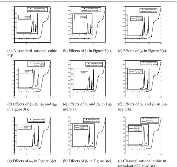
(a) A standard rational cubic FIF.

(b) Effects ofξin Figure (a). (c) Effects ofξin Figure (a).

(d) Effects ofξ,ξ,ξandξ

in Figure (a).

(e) Effects ofαandβin

Fig-ure (a).

(f ) Effects ofαandβin

Fig-ure (b).

(g) Effects ofαin Figure (c). (h) Effects ofβin Figure (c). (i) Classical rational cubic

in-terpolant of Figure (g).

Figure 3 Monotonicity preserving rational cubic FIFs and their derivatives.

(, ), (, ), (, )}. TheC_{-rational cubic FIFs are generated iteratively (Figures} (a)-(i)) as the fixed points of rational cubic IFS (). Sincei=  fori= , , . . . , ,ξi=  for i= , , . . . , , and there is no need to chooseαiandβi, consequently there is no need to

calculateγifori= , , . . . ,  using equation (). The derivatives valuesdi(i= , , . . . , )

are approximated by the arithmetic mean method [] asd= ,d= ,d= ,d= ,

d= ,d= .,d= .,d= .,d= ,d= ., andd= .. Let κ = . in equation (). The scaling factors are restricted asξ∈[, .],

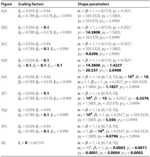
Table 3 Rational IFS parameters for monotonic fractal interpolants

Figure Scaling factors Shape parameters

3(a) ξ6= 0.034,ξ7= 0.44,

ξ8= 0.789,ξ9= 0.578,ξ10= 0.999

αi=βi= 1,i= 6(1)10,γ6= 4.2927, γ7= 503.3320,γ8= 1.5805, γ9= 20.5370,γ10= 2.4994

3(b) ξ6= 0.034,ξ7=0.1,

ξ8= 0.789,ξ9= 0.578,ξ10= 0.999

αi=βi= 1,i= 6(1)10,γ6= 4.2927, γ7=14.3808,γ8= 1.5805, γ9= 20.5370,γ10= 2.4994

3(c) ξ6= 0.034,ξ7= 0.44,

ξ8= 0.789,ξ9=0.1,ξ10= 0.999

αi=βi= 1,i= 6(1)10,γ6= 4.2927, γ7= 503.3320,γ8= 1.5805, γ9=9.6296,γ10= 2.4994

3(d) ξ6= 0.034,ξ7=0.1, ξ8=0.1,ξ9=0.1,ξ10=0.1

αi=βi= 1,i= 6(1)10,γ6= 4.2927, γ7=14.3808,γ8=1.4227, γ9=20.537,γ10=2.0408

3(e) ξ6= 0.034,ξ7= 0.44,

ξ8= 0.789,ξ9= 0.578,ξ10= 0.999

αi=βi= 1,i∈ {6, 7, 8, 10},α9=104,β9=10, α10= 1,β10= 1,γ6= 4.2927,γ7= 503.3320, γ8= 1.5805,γ9=1.1857,γ10= 2.4994

3(f ) ξ6= 0.034,ξ7=0.1,

ξ8= 0.789,ξ9= 0.578,ξ10= 0.999

αi=βi= 1,i∈ {6, 8, 9, 10},

α7=104,β7=10,γ6= 4.2927,γ7=6.3276, γ8= 1.5805,γ9= 20.5370,γ10= 2.4994

3(g) ξ6= 0.034,ξ7= 0.44,

ξ8= 0.789,ξ9=0.1,ξ10= 0.999

αi=βi= 1,i∈ {6, 7, 8, 10},

α9=104,β9= 1,γ6= 4.2927,γ7= 503.3320, γ8= 1.5805,γ9=5.556,γ10= 2.4994

3(h) ξ6= 0.034,ξ7= 0.44,

ξ8= 0.789,ξ9=0.1,ξ10= 0.999

αi=βi= 1,i∈ {6, 7, 8, 10},

α9= 1,β9=104,γ6= 4.2927,γ7= 503.3320, γ8= 1.5805,γ9=4.0796,γ10= 2.4994

3(i) ξi=0,i= 6(1)10 αi=βi= 1,i∈ {6, 7, 8, 10},

α9= 104,β9= 1,γ6=0.0003,γ7=0.0011, γ8=0.0001,γ9=5.0004,γ10=0.0002

of Figure (e) and Figure (a), we notice perceptible variations in the ninth subinterval, and variations in other subintervals are negligible. Again analyzing Figure (a), Figure (c), and Figure (e), we observe that to get appropriate deviations in the rational cubic FIF in the ninth subinterval, one has to vary the scaling parameterξ, the shape parametersα and/orβsuitably.

Next a monotonic rational FIF in Figure (f ) is constructed as per the data in Table  and the variations in [x,x] of Figure (f ) with respect to Figure (a) are more evident than those of Figure (f ) with respect to Figure (b). So, we can say that the scaling factor ξis dominant over the shape parametersαandβin this case at [x,x]. Hence, for ma-jor changes at [x,x], one has to modifyξ, and for minor changes (or fine tuning), one has to alterαand/orβ. This observation is useful for aesthetic requirements in various engineering design problems. By analyzing Figures (g)-(h) with respect to Figure (c), we have noticed that the graphs of rational cubic FIFs in the ninth subinterval in Figures (g)-(h) are concave and convex, respectively. Finally, we construct the classical rational cubic interpolant in Figure (i) with respect to the shape parameters of Figure (g), andξi= 

for alli. Since the shape parametersαandβare the same in Figure (g) and Figure (i), there is some visual similarity between these two curves in [x,x], whereas the same ef-fects are missing in Figure (h) due to a variation inβ. Also, one gets a classical rational cubic interpolant which is similar to Figure (h) in our fractal scheme, wheneverξi= 

Table 4 Uniform errors betweenand rational fractal interpolants, and their derivatives

Monotonic RCFIF

Uniform distance with monotonic RCFIF in Figure 3(a)

Derivative of monotonic RCFIF

Uniform distance with derivative in Figure 3(a)

Figure 3(b) 0.7871 Figure 3(b) 18.736

Figure 3(c) 2.3678 Figure 3(c) 27.0239

Figure 3(d) 2.3783 Figure 3(d) 44.6254

Figure 3(e) 0.8223 Figure 3(e) 3.6775

Figure 3(f ) 2.0038 Figure 3(f ) 18.6884

Figure 3(g) 4.6438 Figure 3(g) 29.531

Figure 3(h) 1.5456 Figure 3(h) 23.4984

Our construction gives an extra freedom for aesthetic modifications in local shape over the classical rational cubic interpolants to an user. For a qualitative study of the derivatives of monotonic fractal interpolants, the readers are invited to check the effects of rational IFS parameters in Figures (a)-(g). The uniform errors between monotonic fractal inter-polants and their derivatives are given in Table  to show the importance of our rational cubic IFS ().

From the examples in Sections -, it is observed that proper interactive adjustments of the scaling factors and shape parameters give us a wide variety of positivity and/or monotonicity preserving fixed points of our rational cubic IFS () that can be used in various scientific and engineering problems for aesthetic modifications. In order to get an optimal choice of the fixed point of our rational cubic IFS (), one can employ a genetic algorithm interactively until the desired accuracy is obtained with the original function.

6 Conclusion

A new type of rational cubic IFS with -shape parameters is introduced in this work such that its fixed point can be used for shaped data. The developed FIF in this paper includes the corresponding classical rational cubic interpolant as a special case. An upper bound of uniform error between the rational cubic FIFψand an original functioninC[x,xn]

is estimated, and consequently we have found thatψconverges uniformly toash→. When the accurate derivatives ofO(hp_i),i= , , . . . ,nare available, and the scaling factors are chosen as|ξi|<κapi–,i= , , . . . ,n– , it is possible to getO(hp) (p= , , )

conver-gence for the rational cubic FIF. Automatic data dependent restrictions are derived on the scaling factors and shape parameters of rational cubic IFS so that its fixed point pre-serves the positivity or monotonicity features of a given set of data. The effects of a change in the scaling factors and shape parameters on the local control of the shape of rational cubic FIF are demonstrated through various examples. Our rational cubic FIFs are more flexible and more suitable for shape related problems in computer graphics, CAD/CAM, CAGD, medical imaging, finance, and engineering applications, and apply equally well to data with or without derivatives. In particular, the proposed method will be an ideal tool in shape-preserving interpolation problems where the data set originates from a positive and/or monotonic function∈C, but its derivativeis a continuous and nowhere dif-ferentiable function.

Competing interests

The authors declare that they have no competing interests.

Authors’ contributions

Author details

1_{Department of Mathematics, Indian Institute of Technology Madras, Chennai, 600036, India.}2_{Department of} Mathematics, Texas A&M University - Kingsville, 700 University Blvd, Kingsville, TX 78363-8202, USA. 3_{Department of} Mathematics, Faculty of Science, King Abdulaziz University, Jeddah, 21589, Saudi Arabia.

Acknowledgements

AKBC is thankful to the Department of Science and Technology, Govt. of India for the SERC DST Project No. SR/S4/MS: 694/10. The authors are grateful to the anonymous referees for the valuable comments and suggestions, which improved the presentation of the paper.

Received: 2 July 2013 Accepted: 16 December 2013 Published:27 Jan 2014

References

1. Mandelbrot, BB: Fractals: Form, Chance and Dimension. Freeman, San Francisco (1977) 2. Feder, J: Fractals. Plenum Press, New York (1988)

3. West, BJ: Fractals in Physiology and Chaos in Medicine. World Scientific, Singapore (1990)

4. Yang, YJ, Baleanu, D, Yang, XJ: Analysis of fractal wave equations by local fractional Fourier series method. Adv. Math. Phys.2013, Article ID 632309 (2013)

5. Hutchinson, JE: Fractals and self similarity. Indiana Univ. Math. J.30, 713-747 (1981) 6. Barnsley, MF: Fractals Everywhere. Academic Press, Orlando, Florida (1988) 7. Barnsley, MF: Fractal functions and interpolation. Constr. Approx.2, 303-329 (1986)

8. Barnsley, MF, Harrington, AN: The calculus of fractal interpolation functions. J. Approx. Theory57, 14-34 (1989) 9. Chand, AKB, Kapoor, GP: Generalized cubic spline fractal interpolation functions. SIAM J. Numer. Anal.44(2), 655-676

(2006)

10. Chand, AKB, Navascués, MA: Generalized Hermite fractal interpolation. Rev. Acad. Cienc. Exactas, Fís.-Quím. Nat. Zaragoza64, 107-120 (2009)

11. Chand, AKB, Navascués, MA: Natural bicubic spline fractal interpolation. Nonlinear Anal.69, 3679-3691 (2008) 12. Chand, AKB, Viswanathan, P: Cubic Hermite and cubic spline fractal interpolation functions. AIP Conf. Proc.1479,

1467-1470 (2012)

13. Chand, AKB, Viswanathan, P: A constructive approach to cubic Hermite fractal interpolation function and its constrained aspects. BIT Numer. Math.53(4), 841-865 (2013)

14. Schmidt, JW, Heß, W: Positivity of cubic polynomials on intervals and positive spline interpolation. BIT Numer. Math.

28, 340-352 (1988)

15. Fritsch, FN, Carlson, RE: Monotone piecewise cubic interpolation. SIAM J. Numer. Anal.17, 238-246 (1980) 16. Schumaker, LL: On shape preserving quadratic spline interpolation. SIAM J. Numer. Anal.20, 854-864 (1983) 17. Brodlie, KW, Butt, S: Preserving convexity using piecewise cubic interpolation. Comput. Graph.15, 15-23 (1991) 18. Späth, H: Spline Algorithms for Curves and Surfaces. Utilias Mathematica Pub. Inc., Winnipeg (1974)

19. Delbourgo, R, Gregory, JA: Shape preserving piecewise rational interpolation. SIAM J. Sci. Stat. Comput.6, 967-976 (1985)

20. Sarfraz, M, AL-Muhammed, M, Ashraf, F: Preserving monotonic shape of the data using piecewise rational cubic functions. Comput. Graph.21, 5-14 (1997)

21. Sarfraz, M, Hussain, MZ, Hussain, M: Shape-preserving curve interpolation. Int. J. Comput. Math.89, 35-53 (2012) 22. Kwakernaak, H, Sivan, R: Linear Optimal Control Systems. Wiley-Interscience, New York (1972)

23. Gregory, JA, Delbourgo, R: Piecewise rational quadratic interpolation to monotonic data. IMA J. Numer. Anal.2, 123-130 (1982)

24. Gregory, JA, Delbourgo, R: Determination of derivative parameters for a monotonic rational quadratic interpolant. IMA J. Numer. Anal.5, 397-406 (1985)

25. Chand, AKB, Vijender, N: Monotonicity preserving rational quadratic fractal interpolation functions. Adv. Numer. Anal.

2014, Article ID 504825 (2014)

26. Akima, H: A new method of interpolation and smooth curve fitting based on local procedures. J. Assoc. Comput. Mach.17, 589-602 (1970)

10.1186/1687-1847-2014-30

Cite this article as:Chand et al.:Rational iterated function system for positive/monotonic shape preservation.