Delay allocation between source buffering and interleaving for wireless video

R E S E A R C H

Open Access

Delay allocation between source

buffering and interleaving for wireless video

Yushi Shen

, Kartikeya Mehrotra

, Pamela C. Cosman

, Laurence B. Milstein

and Xin Wang

Abstract

One fundamental tradeoff in the cross-layer design of a communications system is delay allocation. We study delay budget partitioning in a wireless multimedia system between two of the main components of delay: the queuing delay in the source encoder output buffer and the delay caused by the interleaver. In particular, we discuss how to apportion the fixed delay budget between the source encoder and the interleaver given the channel characteristics, the video motion, the delay constraint, and the channel bit rate.

Keywords: Delay budget partitioning, Delay constraint, Cross-layer optimization, Video communications, Wireless video

Abbreviations: BER, Bit error rate; BPSK, Binary phase shift keying; bps, Bits per second; CDF, Cumulative distribution function; DCT, Discrete cosine transform; FEC, Forward error coding; fps, Frames per second; LDPC, Low-density parity check; MB, Macroblock; MC, Motion compensated; MCTF, Motion- compensated temporal filtering; MSE, Mean square error; PSNR, Peak signal-to-noise ratio; QCIF, Quarter common intermediate format; RCPC, Rate-compatible punctured convolutional code; TMN, Test model number

1 Introduction

Delay partitioning is a fundamental tradeoff problem in the cross-layer design of a communications system. This problem is especially important in real-time video communications such as video conferencing or video tele-phony, in which there exists a tight end-to-end delay con-straint. For example, interactive video telephony should have a maximum end-to-end delay of no more than around 300 ms. Once the receiver begins displaying the received video, the display process must continue without stalling. In other words, in order to be useful, frame data entering the source encoder at timetmust be displayed at the decoder by time(t+T), whereT is the delay con-straint, that is, an upper bound for end-to-end delay of the system. In addition, the available data rate on the channel is constrained by the available bandwidth.

In [1] and [2], the design of rate-control schemes for low-delay video transmissions was studied for a noise-less channel. In [3] and [4], the efficient design of an interleaver for a fading channel was investigated. In [5],

*Correspondence: [email protected] 4VMware Inc., Palo Alto, CA 94304, USA

Full list of author information is available at the end of the article

specific tandem and joint source-channel coding strate-gies with complexity and delay constraints were ana-lyzed and compared. In [6–8], delay-constrained wireless video transmission schemes were proposed for different application scenarios. In [9] and [10], tradeoffs between delay and video compression efficiency were discussed for a motion-compensated temporal filtering (MCTF) video codec and for hierarchical bi-directional (B-frames) schemes, respectively. In [11], the tradeoff between the long-term average transmission power and the average buffer delay incurred by the traffic was analyzed math-ematically over a block-fading channel with delay con-straints. And in [12], the tradeoff between the network capacity and the end-to-end queueing delay was studied for a mobile ad hoc network.

In this literature, either design strategies with delay con-straints were investigated without considering any trade-off issue, or certain tradetrade-off problems with delay con-straint were discussed for different purposes and contexts than those in this paper. In this paper, we study delay par-titioning for video communications over a Rayleigh fading channel. In particular, we focus on the delay allocation between the source encoder buffer and the interleaver as we vary various parameters, such as the motion of the

video content, the rate of variation of the channel, the end-to-end delay constraint, the channel bit rate, and the channel code rate.

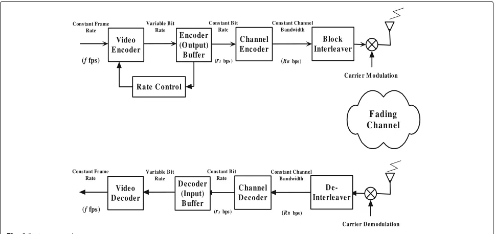
The system model we study is shown in Fig. 1. Typically, video frames arrive at the video encoder at a constant frame rate. The frames are compressed to a variable bit stream and passed on to the video encoder output buffer from which bits are drained at a constant rate. To pro-tect against channel errors, forward error coding (FEC) is employed on the compressed bitstream coming out of the encoder buffer. This is followed by interleaving to provide robustness to channel fading. Finally, the bit stream com-ing out of the interleaver is modulated and sent over the wireless channel. At the receiver, the bitstream is demod-ulated, de-interleaved, decoded, and then passed on to the video decoder input buffer (henceforth called the decoder buffer). The video decoder extracts bits from the decoder buffer at a variable rate to display each frame at its cor-rect time and at the same constant frame rate at which they were available to the video encoder. A rate-control mechanism is used at the video encoder to control the number of bits allotted to each frame so that the encoder buffer and the decoder buffer never overflow or under-flow, while maintaining acceptable video quality at all times. Note that we assume there is no video encoder input buffer, and no video decoder output buffer; hence, the video encoder output buffer and the video decoder input buffer are called the encoder buffer and decoder buffer, respectively, throughout this paper.

The paper is organized as follows. In Section 2, the system model is introduced in detail. In Section 3, we formulate the delay partitioning problem mathematically

and end up with a relationship among source encod-ing buffer delay, interleavencod-ing delay, and channel decodencod-ing delay, under a delay constraint. Simulation results of the tradeoff between the source encoder buffer and the inter-leaver are shown and analyzed in Section 4, for different video sequences over Rayleigh fading channels. In partic-ular, we study how the tradeoff will be affected by the motion of the video content, the rate of variation of the channel, the delay constraint, and the channel bit rate. Lastly, Section 5 concludes the paper.

2 System model with delay constraint

In this section, we will discuss the components in Fig. 1 in detail.

2.1 Source coding

In real-time video communications, the end-to-end delay for transmitting video data needs to be very small, par-ticularly for interactive two-way applications such as video conferencing and gaming. Video data enters the source encoder at a constant rate of f frames per sec-ond (fps), where it first undergoes block-based motion-compensated (MC) prediction, followed by DCT trans-formation of the residual block. The DCT coefficients are quantized by appropriately choosing the quantization parameter, and the quantized values are then run-length and Huffman coded. Assume the transmission bit rate is RBbits per second (bps), and the source-coded bit stream leaves the encoder buffer atrsbps.

Whenever a frame occupies more than rs/f bits, bits will accumulate in the source encoder buffer and increase the encoder buffer delay experienced by the incoming bits.

If this trend continues for several frames, the buffer may fill up because the buffer size is limited. When the num-ber of bits in the buffer is more than a predetermined threshold, it will lead to frame skipping as will be dis-cussed later. On the other hand, whenever a frame occu-pies less thanrs/f bits, the encoder buffer fullness level decreases. If this trend continues for several frames, the encoder buffer may run empty, thereby wasting channel bandwidth.

By sensing the buffer fullness and keeping an estimate of the available bit budget, the rate control chooses the quan-tization step size and seeks to prevent buffer overflow and underflow while maintaining acceptable video quality. If either the remaining bit budget is small or the buffer is getting full, the rate control resorts to coarse quantization. If either the remaining bit budget is large or the buffer is getting empty, the quantization step size is reduced (i.e., fine quantization). A large delay budget for the source encoder allows the use of a large encoder buffer, which tends to result in higher-quality video because the rate control has more freedom. Typically, the increased num-ber of bits resulting from finely encoding a complex scene can be easily accommodated in the large buffer. However, when tight delay constraints exist, the system must oper-ate with a small encoder delay budget, or equivalently a small encoder buffer, which tends to reduce the quality of the video, as the functioning of the rate control is more constrained. In extreme cases, the encoder buffer may fill up several times, leading to loss of data through repeated frame skipping.

On the decoder side, the incoming stream of video data is buffered in a source decoder buffer. Once the source decoder starts displaying the frames, the delay constraint becomes operational. IfT denotes the upper bound for end-to-end delay of the system, a frame entering the encoder at timetmust be displayed at the decoder at time (t+T), and all the video data corresponding to this partic-ular frame must be available at the decoder accordingly. A video frame that is not able to meet its delay constraint is useless and is considered lost. We assume that the source decoder has knowledge of the frame numbers skipped by

the source encoder and that it holds over the immediately preceding displayed frame and displays it in place of the skipped frame.

In H.263, the rate control performs the bit allocation by selecting the encoder’s quantization parameter for each block of 16×16 pixels. We choose the test model number 8 (TMN-8) rate control [1, 2] recommended for low-delay applications. The TMN-8 rate control is a two-step approach: a frame layer control first selects a target bit count for the current frame, followed by a macroblock (MB) layer rate control which selects the quantization step size for each MB in the frame. The TMN-8 rate control has a threshold for frame skipping. Whenever the number of bits in the encoder buffer increases beyond this threshold, typically one frame is skipped so that the number of bits in the buffer falls below the threshold. For each skipped frame, buffer fullness reduces byrs/f bits. We assume the first frame in the video sequence is coded as anI frame, and all subsequent frames asPframes, since this is a com-mon strategy for video communications with a tight delay budget. We also assume theI frame is transmitted error free to the decoder and the decoder does not start the dis-play until the firstIframe is completely buffered. The rate control starts with the firstPframe. Once theI frame is displayed, the delay constraint becomes operational and all subsequent frames must meet their delay constraint.

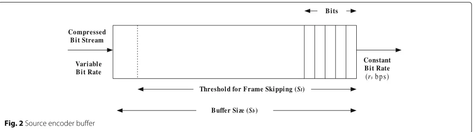
From the point of view of the system engineer, the parameter of interest is the threshold for frame skipping (denoted bySt). However, for the hardware engineer, the buffer size (denoted Sb) is more important. These two quantities are closely related, as explained now. As shown in Fig. 2, we modify the rate control such that, while encoding the frame, if the buffer fullness level exceedsSt, the remaining MBs of the frame are all skipped. If a par-ticular sequence comprisingNskipbits is used to inform the decoder of this situation, the buffer size required is Sb=St+Nskip. BecauseNskipis usually much smaller than St, for exampleNskip=24 in our system whileStis at least several thousand, for simplicity, we assume the threshold for frame skipping and the buffer size are the same and are equal toS, i.e.,Sb=St=S.

2.2 Channel coding

The information bitstream coming out of the source encoder buffer is channel coded using a rate-compatible punctured convolutional (RCPC) code with rate rc and constraint lengthν[13]. At the receiver, the Viterbi algo-rithm is used to find the best candidate in the trellis for the received bitstream. The delays encountered in the chan-nel encoder and decoder are called the chanchan-nel encoding delay and the channel decoding delay. Together, these make the delay budget of channel coding. When using a convolutional code with constraint lengthν, the chan-nel decoding delay is approximately the decision depth of the Viterbi decoder, which is about 5νin bits. The deci-sion depth for punctured convolutional codes is generally longer. If the puncturing period for the RCPC code is P, the decision depth can be bounded by 5Pν [14]. We note, however, that when using channel encoding schemes such as turbo coding that require iterative decoding at the receiver, the channel coding delay budget may use up a significant portion of the overall delay budget.

Bandwidth is a major resource shared between source coding and channel coding. A bandwidth constraint limits the available rate on the channel. Allocating more band-width to the source encoder allows more information from the source to be transmitted, resulting in better-quality video. However, the bandwidth available for chan-nel coding is reduced, leading to increased errors on the channel and thus a reduced probability of achieving high video quality. Let RB bps be the total available rate on the channel, and rs and rc be the average source cod-ing rate and the channel code rate, respectively. Then the bandwidth constraint is expressed as [15, 16]

rs rc =

RB. (1)

2.3 Interleaving and fading channel model

We consider coherent BPSK over a flat fading channel, where flat fading means that there is a constant gain across the bandwidth of the received signal. Therefore, the effect of the channel is a multiplicative gain term on the received signal level. We use the channel model suggested by Jakes [17], in which the envelope of the fading pro-cess is assumed to be Rayleigh distributed. The Doppler spectrum is given by

S(f)= 1

1−(f/fD)2, (2)

wherefD is the Doppler frequency and is given byfD = fcv/c, where fc is the carrier frequency,v is the mobile velocity, andcis the speed of light. The covariance func-tion of the fading process for this channel model can

be shown to be given by the first order Bessel function, namely

Rα(τ)=J0(2πfD|τ|), (3)

whereτ is the time separation between the two instances when the channel is sampled. Thus, the correlation between two consecutive symbols with separationTs is J0(2πfDTs), whereTsis the symbol time. The productfDTs is usually called the normalized Doppler frequency.

Error control coding works well when the code symbols used in the decoding process are affected by indepen-dent channel conditions. Correlated fading is one of the sources of channel memory on the land mobile channel. Interleaving is used to break up channel memory, and it is an essential element in the design of error control coding techniques for the land mobile channel. A block inter-leaver formats the encoded data in a rectangular array of N1rows andN2columns. The code symbols are written in row-by-row and read out column-by-column. On the decoder side, the received symbols are first de-interleaved before they enter the decoder. As a result of this reorder-ing, the fading samples of two consecutive symbols enter-ing the decoder are actuallyN1Ts apart in time, and the correlation between two consecutive channel instances is now given as J0(2πfDN1Ts). The parameter N1 is often referred to as the depth of the interleaver.

The inverse of the normalized Doppler frequency roughly equals the coherence time,Ncoh = 1/(fDTs), of the channel in bits, and is a measure of the number of con-secutive bits over which the channel remains correlated. The amount of interleaving required depends on the chan-nel. If the channel is slower, the coherence time is larger and consequently a larger interleaver is required. When there is no limit on the size of the interleaver, perfect interleaving can be achieved for mobile channels, which ensures that the fading envelopes are uncorrelated. How-ever, both interleaving and de-interleaving introduce delay in the system, called the interleaving delay. Both of these delays are equal toN1N2Tsseconds. In a practical system, the interleaving delay budget is constrained not only by the overall delay budget but also by the delay budget nec-essary for the robust functioning of the source coding and the channel coding.

chosen slightly larger than the length of the shortest error event of the code.

Interleaving, in conjunction with FEC, is a mechanism to achieve time diversity, where, by transmitting con-secutive symbols sufficiently separated in time, nearly independent fading is ensured. As with any diversity tech-nique, the performance improvement shows diminishing returns with increased diversity order. Note that the effec-tive order of diversity is a nondecreasing function ofN1. Various rules of thumb are available in the literature to determine the interleaver depth sufficient to extract nearly independent fading case performance [3, 4].

In [3], simulations were used to demonstrate that fully interleaved performance is approximately achieved for BPSK over exponentially correlated channels when the interleaver depth is chosen to satisfyfDTsN1 > 0.1. This rule, however, does not apply to correlated fading chan-nels with other auto-correlations, such as Jakes’ model. In [4], a simple figure of merit for evaluating the depth of the interleaver was obtained for Rician channels, and a variety of channel auto-correlation functions. However, as shown in our simulations, this figure of merit does not hold true for Jakes’ fading model with lowκ factor (κ is the ratio of signal energy in direct and diffused signal components) Rician channels and the limiting Rayleigh fading case.

3 The delay constraint formulation

The end-to-end delay constraint of each frame,T, is the upper bound to the delay that a frame may experience and still be able to be displayed on time, where by delay, we mean the time difference between when the video frame is captured for encoding and when it reaches the video decoder. Consider frame i captured at time t. Without loss of generality, we assume t to be zero. Further, we assume that each frame has the same number of MBs, and denote this number byM(e.g., for video with QCIF format, M = 99). We also denote the MB index by k (k=0, 1, 2,· · ·,M−1), and we letbi(k)be the number of bits in thekth MB of theith frame.

Frames arrive at the video encoder at some constant frame rate, and thus, the processor has to process each frame in the same amount of time because we assume there is no video encoder input buffer. Each frame has the same number of MBs, and we assume each MB has to be processed in the same amount of time. At the video decoder, frames are displayed at a constant frame rate, and we assume there is no video decoder output buffer.

For frameito meet its delay constraint, the kth MB’s decoding must begin at timeT−(M−k)Td, whereTdis the time required to decode a MB (source decoding only, i.e., excluding the FEC decoding) and is assumed to be the same for all MBs. Also, thekth MB becomes available for encoding only after timekTe, where Te is the encoding time of a MB (source encoding only, i.e., excluding the FEC

encoding) assumed to be the same for all MBs. Thus, if thekth MB is to meet its decoding deadline, the following must be true:

Teb(k) + Tenc(k)+Tint(k)+Tc(k)+TCH + Tdein(k)+Tdec(k)+Tdb(k)

=T−(k+1)Te−(M−k)Td, (4)

whereTeb(k)is the encoder buffer delay, i.e., the time the kth MB waits in the encoder buffer before it starts moving out to the channel encoder,Tenc(k)is the FEC encoding delay for thekth MB,Tint(k)is the delay caused by inter-leaving for the kth MB, Tc(k) is the transmission time for the kth MB, TCH is the channel propagation delay, assumed to be a known constant, Tdein(k) is the delay caused by de-interleaving for thekth MB,Tdec(k) is the channel decoding delay, and finallyTdb(k)is the decoder buffer delay for thekth MB, i.e., the time it waits in the decoder buffer before its decoding begins for display.

can be neglected. Assuming a constant channel propaga-tion delayTCH, and noting that we needTdb(k) > 0 to guarantee the source decoder buffer does not run empty, Eq. (5) can be rewritten as

Teb(k)+ 2N

RB + 5Pν

RB ≤

C, (6)

whereC=T−(M+1)TMB−TCH, is a constant. The encoder buffer delay experienced by each MB in each frame must satisfy the above inequality in order for the corresponding frame to meet its display deadline. As explained previously, the maximal number of source coded bits in the source encoder buffer is equal toS, and they leave the buffer at a ratersbps; thus,Teb(k) ≤ S/rs. As a result, Eq. (6) is always true whenever the following is true:

S rs +

2N RB +

5Pν RB =

C, (7)

whereS/rs can be viewed as the delay budget for source coding, 2N/RB as the delay budget for interleaving and 5Pν/RB as the delay budget for channel decoding. As a result, the delay partitioning problem is to allocate the delay budget among these three components under the constraint (7), such that the overall distortion of the video transmission is minimized. In the following section, sim-ulation results are presented to study the three main com-ponents in the delay budget. A possible future research interest may be to apply some analytical models with suit-able utility function computed from the three delay budget

components, so that the delay budget tradeoffs can be resolved analytically in some specific conditions, but that would be beyond the scope of this paper.

4 Simulation results and discussion

4.1 The effect of interleaver depth on system performance

An interleaver is important to remove the channel mem-ory when error control codes designed for memmem-oryless channels are applied to channels with memory. Before we consider the tradeoff in delay allocation in wireless multimedia, we first study the effect of interleaver design without a delay budget restriction.

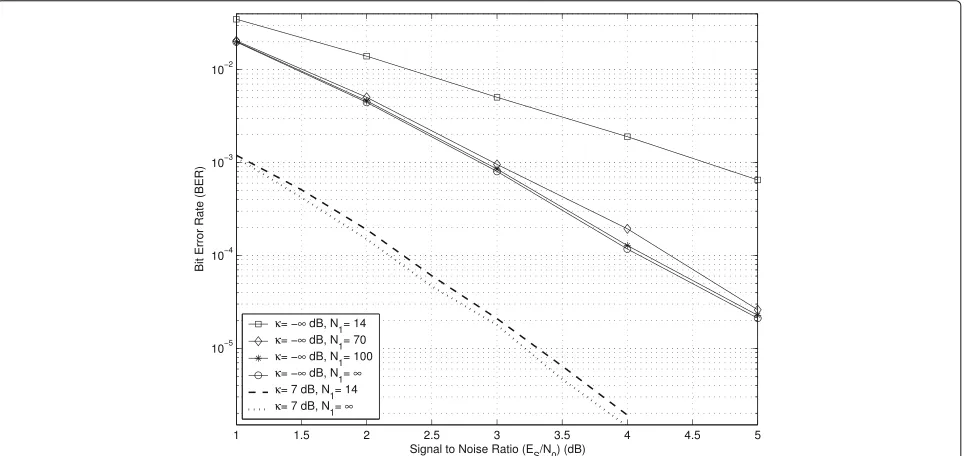
The performance of an interleaver is governed by its interleaving depth N1. As mentioned in Subsection 2.3, simulation results in [3] demonstrated that fully inter-leaved performance is approximately achieved for BPSK over exponentially correlated channels when N1 ≥ 0.1Ncohis satisfied, and [4] further extended this result to Rician channels and a variety of channel auto-correlation functions by proposing a simple figure of merit for eval-uating interleaver depth. Our simulations confirm this result for Jakes’ fading model with high κ factor Rician channels. In Fig. 3, we show simulation results for a system with a channel code of raterc=1/2 and minimal distance dmin = 10, an interleaver withN2 = 100 columns, and Jakes’ fading spectrum withfDTs =0.01. The two bottom dashed lines are drawn for the Rician channel withκ =5 (or 7 dB), with interleaver depthN1=14 and ideal inter-leaving (i.e., N1 = ∞). These results match the results

of Fig. 4 in [4], which illustrates thatN1 = 14, which is slightly larger than 0.1Ncoh=10, gives performance close to ideal (infinite) interleaving.

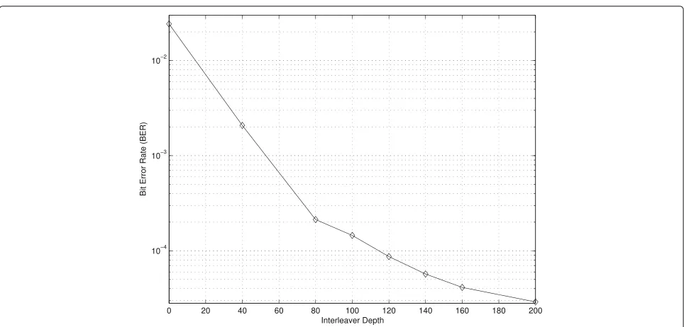
However, further simulations illustrate that this figure-of-merit does not hold true for Jakes’ fading model with low κ factor Rician channels. Lowering the κ factor of the Rician channel makes the fading more severe, and the channel is Rayleigh whenκ = 0 (or−∞dB), where the direct signal component is totally absent. Clearly with decreasingκ, the performance degrades and a larger inter-leaver depth may be required. In Fig. 3, the performance whenκ =0 is shown, by utilizing interleavers with depth N1 = 14,N1 = 0.7,Ncoh = 70,N1 = Ncoh = 100, and infinite interleaving. As seen from the four top plots, sub-stantial gains in performance are achieved overN1= 14, with an improvement by an order of magnitude, especially at middle and high SNR. On the other hand, although the performance improves significantly fromN1 = 14 to N1 = 70, there is not much gain in further increasing after N1 ≥ 70. This is the typical characteristic of any diversity system, where with increasing diversity order, the improvement in performance shows diminishing returns. Figure 4 further illustrates this point, by showing bit error performance versus interleaver depth, with a convo-lutional channel code havingrc = 1/3, constraint length ν=6, anddmin=14 [13, 21], over a Rayleigh fading chan-nel withfDTs =0.005 (i.e.,Ncoh =200).N2is fixed to be 16, which is slightly greater thandmin[18, 19]. We again note the sharp fall in bit error rate (BER) asN1increases from 0 to 80, and that the performance begins to flatten

out aroundN1 = 140 onwards, which is again the depth corresponding to 0.7Ncoh.

As a result, our simulation results suggest the following: for Rician channels with high κ factor, fully interleaved performance is approximately achieved when the inter-leaver depthN1≥0.1Ncoh; while for Rician channels with lowκ factor, in particular for a Rayleigh fading channel, fully interleaved performance is approximately achieved whenN1 ≥ 0.7Ncoh. Also, the number of columns (N2) should be greater than the minimal distance (dmin) of the channel code to avoid the wrap around effect.

4.2 Delay allocation between the source encoder buffer and the interleaver, for fixed delay budget, channel bit rate, and FEC code

We will discuss the delay allocation between the source encoder buffer and the interleaver in this and the next subsections. In all our simulations, we encoded QCIF size video sequences atf =10 fps. Also, for all comparisons, we kept the ratio of the energy-per-coded bit to the noise power spectral density,Es/N0, constant at 3 dB. For each set of system and channel parameters, we ran 10,000 real-izations of the time-correlated Rayleigh fading channel, which were generated using Jakes’ model [17]. We com-puted the cumulative distribution function (CDF) of the average peak signal-to-noise ratio (PSNR), where PSNR is calculated by first averaging the mean square error (MSE) for the entire decoded video sequence, and then convert-ing to PSNR. The system performance can be gauged once the CDF curves for each possible set of parameters in the

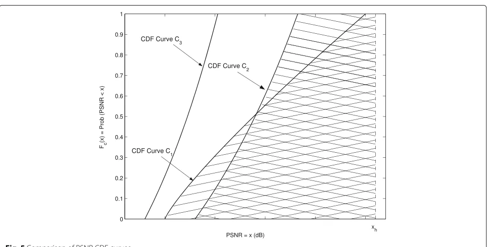
set of interest are available. For example, Fig. 5 illustrates what the CDF curves could look like. Whenever two CDF curves do not intersect (e.g., curvesC1andC3in Fig. 5), the lower curve is superior because it always has a higher probability of achieving any given average PSNR. When there are crossovers between two curves (e.g., curvesC1 and C2 in Fig. 5), then one curve may be superior for one application but not for another. Comparison between the curves may then involve criteria such as minimizing the area under the curve, perhaps with some weighting. In this paper, as shown in Fig. 5, to evaluate the sys-tem performance, we adopted the criterion from [22] of minimum area under the CDF curve to the left of a cer-tain thresholdx_hdefined later in the paper, i.e., the value

xh

0 Fc(x)dx.

In this subsection, we analyze the delay partition between the source encoder buffer and the interleaver, for a fixed delay budgetC, a given channel bit rateRBand a fixed RCPC code with raterc. As explained in Section 2, the delay budget of the source encoder is determined by the threshold for frame skippingS. GivenRBand a RCPC code with rate rc, the source coding rate, rs, is deter-mined by (1), and the channel decoding delay, which is roughly equal to (5Pν/RB), is also fixed. Under this sce-nario, increasing the delay budget of the source encoder comes at the cost of reducing the interleaver delay bud-get, i.e., using a smaller interleaver. In general, given the total delay budgetCand channel bit rateRB, the choice of Sis affected by the source encoding ratersand the video content, and the choice of interleaver depthN1is related to the channel fading characteristics (Ncoh and channel

model) and the video content. Therefore, we will focus on how this tradeoff will be affected by the motion of the video content, the rate of variation of the channel, the delay constraint and the channel bit rate.

In the following simulations, we used the raterc =1/3 RCPC code withν = 6 anddmin = 14 [13, 21] for chan-nel coding, andN2was fixed at 16. We ran the simulations with different parameters, for example, video sequences with high, medium, or low motion, channels with fast, medium, or slow fading, delay constraints that are tight, medium, or loose , and different channel bit rates.

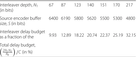
First, we assume a delay constraint C = 150 ms and a channel bit rate RB = 144 kbps (thus rs = 48 kbps). We simulated the system for a medium motion sequence “Foreman” QCIF over a medium fading channel with normalized Doppler frequency fDTs = 0.005 (Ncoh = 200 bits). The candidate delay allocations we tested are summarized in Table 1, which were calculated based on Eq. (7). Figure 6 shows the CDF curves of the PSNRs for these delay allocations, and the areas under the CDF curves are plotted as the solid line in Fig. 7, where the x-axis is the interleaver delay budget expressed as a fraction of the total delay budget. It is seen that, as the inter-leaver delay budget increases fromN1 = 67, the system performance initially improves because of the increased diversity gain. However, the diversity gain shows dimin-ishing returns, and at some point the reduction in source encoder delay budget starts having more of an effect, and the system performance degrades. It is seen that (N1 = 151,S=5500)is the optimal delay allocation for this case, whereN1is about 3₄Ncoh.

Table 1Delay allocations for tradeoff betweenSandN1, used in

the simulations for Figs. 6 and 7

Interleaver depth,N1 (in bits)

67 87 123 140 151 170 217

Source encoder buffer size,S(in bits)

6400 6190 5800 5620 5500 5300 4800

Interleaver delay budget

as a fraction of the 9.93 12.89 18.22 20.74 22.37 25.19 32.15

Total delay budget, ₂

N1N2 RB

/C(in %)

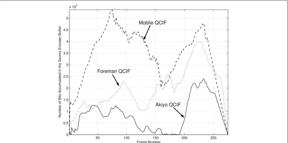
To see the effect of the motion of the video content, we also simulated a very high motion sequence “Mobile” QCIF and a very low motion sequence “Akiyo” QCIF, with the other parameters the same (C = 150 ms, RB = 144 kbps and Ncoh = 200). The system performances measured by the areas under the CDF curves are plotted and compared in Fig. 7, where the threshold valuexhwas set to be the maximal PSNR value observed among all the realizations in the test for that individual video sequence. For example, in Fig. 6, the largest PSNR achieved by any of the systems is 33.01 dB, so for the purposes of gener-ating the curve corresponding to Foreman QCIF in Fig. 7, we compute the areas under the CDF curves and to the left ofxh = 33.01 for the curves in Fig. 6. Because differ-entxhvalues were used for the three curves corresponding to the three different video sequences, the performance comparison (i.e.,y-axis values) is only meaningful within a curve, but not between different curves. It is observed

that, given the above parameters, a higher motion video sequence requires a higher source encoder buffer sizeS, at the cost of a smaller interleaver depth. For example, Fig. 7 shows the optimal choices ofN1are 170, 151, and 140, for Akiyo, Foreman, and Mobile, respectively. In com-pressing video, some frames may need more bits than other frames because of the presence of fine detail. In addition, for a high motion video, some frames may need a significantly larger number of bits than others to well represent the occurrence of high motion, and the perfor-mance may degrade more seriously during concealment for frame skipping. As a result, a larger source encoder buffer is needed. To further illustrate this point, in Fig. 8, we assumed an unconstrained encoder buffer size, and recorded the number of bits accumulated in the buffer for the three video sequences when the source rate was rs = 48 kbps. Note that, although the buffer size is unlimited here, the number of bits accumulated is not infi-nite because the system is still subject to rate control. As expected, Fig. 8 illustrates that a higher motion sequence usually needs a larger buffer size than a lower motion sequence.

We also simulated the system for different channel vari-ation rates, with the sameC=150 ms andRB=144 kbps. Figures 9 and 10 show the performance results for a slowly fading channel withfDTs = 0.0035 (Ncoh = 286 bits), and Figs. 11 and 12 are for a fast fading channel with fDTs =0.01 (Ncoh = 100 bits). Also, Figs. 9 and 11 show the CDF curves of the PSNRs for Foreman QCIF, and Figs. 10 and 12 compare the areas under the CDF curves of

Fig. 7System performance, as measured by the areas under the CDF curves, versus the fraction of the interleaver delay budget, for different video sequences, Rayleigh fading channel withfDTs=0.005, delay budgetC=150 ms, and channel bit rateRB=144 kbps. The curve for Foreman QCIF is derived from Fig. 6 withxh=33.01

all three video sequences. Again, thexhvalues were set to the maximal PSNRs observed for the corresponding video sequences. It is seen that, given the same set of system parameters, a larger N1 is preferable for a slowly fading channel, in order to break the channel memory, whereas a

smallerN1is preferable for a fast fading channel to free up more of the delay budget for the source encoder buffer.

Next, we simulated the system for different delay bud-gets and different channel bit rates. Figure 13 shows the system performance for Foreman QCIF atRB=144 kbps

Fig. 9CDF curves of the PSNRs for various delay allocations, for Foreman QCIF, Rayleigh fading channel withfDTs=0.0035, delay budget C₌150 ms, and channel bit rateRB=144 kbps

and fDTs = 0.005, with a tight delay constraint C = 100 ms, a medium constraint C = 150 ms and a very loose constraint C = 250 ms. In order to compare the performance not only along each curve in Fig. 13, but also across curves, the samexh value, set to be the maximal observed PSNR value in all the simulations for Fig. 13,

was applied for the area calculations. It is seen that, for the three constraints, the optimal choices ofN1are 135, 151, and 180, respectively, while the corresponding opti-mal ratios of the interleaver delay budget to the total delay budget are 30.0, 22.4, and 16.0 %, respectively. In other words, as the delay budgetCincreases, the optimal

Fig. 11CDF curves of the PSNRs for various delay allocations, for Foreman QCIF, Rayleigh fading channel withfDTs=0.01, delay budget C=150 ms, and channel bit rateRB=144 kbps

interleaver depthN1increases, because of more available resources, while the corresponding ratios of the inter-leaver delay to the total delay budget decrease, because of the diminishing returns of the diversity gain. Also, it is seen that the system performance with the best (N1,S) choice improves, i.e., has a smaller area (y-axis value), asC

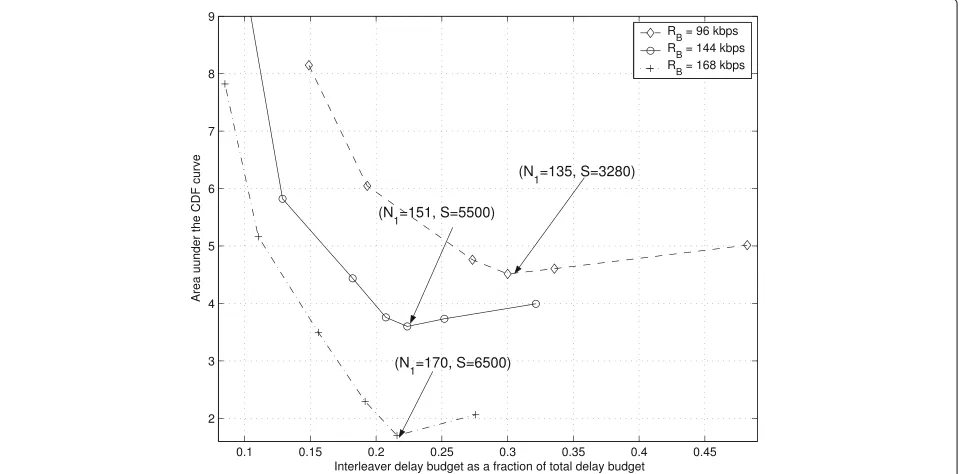
increases. Similar trends occur when the channel bit rate RBincreases, holding other system parameters constant. As shown in Fig. 14, which plots the system performance for Foreman QCIF atC=150 ms andfDTs=0.005, with different channel bit rates, the optimal choices ofN1are 135, 151, and 170, forRB= 96 kbps,RB =144 kbps, and

Fig. 13System performance, as measured by the areas under the CDF curves, versus the fraction of the interleaver delay budget, for delay budgets C₌100 ms,C₌150 ms, andC₌250 ms, Foreman QCIF, Rayleigh fading channel withfDTs=0.005, and channel bit rateRB=144 kbps. All the areas are calculated withxh=34.16, and the curve forC=150 ms is derived from Fig. 6

RB=168 kbps, respectively, and the corresponding ratios of the interleaver delay budget to the total delay budget are 30.0, 22.4, and 21.6 %, respectively. Also, the system performance with best (N1,S) choice improves whenRB increases.

Examining the results shown in figures from Figs. 6 to 12, as well as our other simulation results, we see the fol-lowing trends. First, the normalized Doppler frequency is the key parameter in the delay partitioning, and a sys-tem operating over a fast fading channel prefers a smaller

interleaver depthN1. And as shown in all the above simu-lation results, it seems that about 0.7Ncoh(more precisely, from 0.6Ncohto 0.9Ncoh) is a safe choice forN1. This result is consistent with our conclusion in Subsection 4.1, which illustrates that the maximum gain from the interleaver is approximately achieved whenN1≥0.7Ncohin a Rayleigh fading channel. Second, the video content also affects the delay partitioning; a sequence with higher motion con-tent usually prefers a larger source encoder, and thus a smallerN1. Third, either fast fading, or a larger total delay budget C, or a larger channel bit rateRB, improves the system performance on the average, holding other param-eters the same. For example, Figs. 6, 9, and 11 show that, for a given set of system parameters, the highest PSNR achieved improves from about 32 dB to about 34 dB when the channel varies more rapidly. Note that the perfor-mance improvement for a largerC or a largerRBis due to the system having additional available resources, while the performance improvement for fast fading is due to additional channel diversity. However, the last conclusion is valid only for accurate channel estimation. Lastly, the gaps between the performances of the optimal delay allo-cation and various sub-optimal delay alloallo-cations decrease when the channel varies faster. For example, in Fig. 10 (a slowly fading channel), the performance of the optimal allocation and those of other allocations varies by a factor of 10, while in Fig. 12 (a fast fading channel), the differ-ences are limited to a factor of 1.2. This implies that the delay allocation issue is more important when the chan-nel varies slowly. When the chanchan-nel varies fast enough, different allocations may not affect the performance as much.

4.3 Bandwidth allocation and delay allocation

In this subsection, we vary the channel coding rate, rc, to analyze the bandwidth partition between source cod-ing and channel codcod-ing, together with the delay partition between the source encoder buffer and the interleaver, for a fixed delay budget,C, and a given channel bit rate,RB.

Again, the ratesrsandrc must satisfy bandwidth con-straint (1). Also, we note from delay concon-straint (7) that, for a fixed RB, the interleaver delay, which is equal to 2N/RB, and the channel decoding delay, which is equal to 5Pν/RB, do not change by changingrs. This implies that increasingS proportionately withrs will ensure that the same delay allocation is maintained. However, maintain-ing the same delay allocation is not necessarily desirable. With a change in rs andrc, the optimal delay allocation may change.

Assume there areNccandidate channel codes with rates {rc}. The optimal bandwidth partition and delay partition, i.e., the best (rc,rs,N1,S) 4-tuple, can be determined by a two-step optimization method:

Step I: For each channel code candidate with rate rc, calculate the correspondingrs from Eq. (1). For each (rc,rs) pair, among the candidate delay partition pairs (N1,S), find the one for this bandwidth alloca-tion that minimizes the area under the CDF curve, as illustrated in Section. 4.2. This yieldsNc4-tuples, with corresponding PSNR CDF curves.

Step II: Among theNc4-tuples, find the one with the smallest area under its CDF curve, using a common threshold value,xh. This (rs,rc,N1,S) 4-tuple is the one with best bandwidth and delay allocations.

To illustrate this procedure, we simulated the system for different channel codes in the same RCPC family, with rates equal to 1/3, 4/11, 2/5, and 4/9 [13], for Foreman QCIF atfDTs = 0.005,RB= 144 kbps, andC =150 ms. From Eq. (1), the corresponding source coding rates are 48, 52.4, 57.6, and 64 kbps, respectively. For each (rc,rs) pair, different (N1,S) pairs that satisfied Eq. (7) were sim-ulated, and the (N1,S) pair that minimized the area under the CDF curve was selected. For example, the pair (N1 = 151,S = 5500) was selected for the bandwidth allocation (rc = 1/3,rs = 48 k), where the areas of CDF curves were derived from Fig. 7. In Fig. 15, we show, for four possible (rc,rs) allocations, the CDF curve for the corre-sponding best (N1,S) pair. They are (N1=151,S=5500), (N1 = 170,S = 5780), (N1 = 190,S = 6110), and (N1=217,S =6400), forrc= 1/3,rc =4/11,rc =2/5, andrc =4/9, respectively. Then, the best bandwidth and delay partition 4-tuple was selected among the four candi-dates shown in Fig. 15. In Fig. 16, we plot the areas under all the CDF curves, wherein all curves were calculated with the same threshold xh = 35.78. It is seen that the (rc = 1/3,rs = 48 k,N1= 151,S = 5500) 4-tuple yields the best overall performance.

Fig. 15CDF curves of the PSNRs for the best (N1,S) choices of different channel coding rates {rc}, Foreman QCIF, Rayleigh fading channel with fDTs=0.005, delay budgetC=150 ms, and channel bit rateRB=144 kbps

source encoder and the interleaver, both of which want a larger delay budget. It turns out that the best selection is one that results in a larger S and a larger N1. Fur-ther, the optimal ratio of the interleaver delay to the total delay budget, which is equal to(2N1N2)/(RBC), also

increases, becauseN1increases, whileC,RBandN2are kept constant.

Lastly, Fig. 16 shows that, when increasingrc, the sys-tem performance with the best delay partition degrades. For example, the performance gaps between that of the

optimal delay allocation forrc = 1/3 and those forrc = 4/11,rc = 2/5, andrc = 4/9, are about a factor of 0.34, 2.50, and 8.81, respectively. It is seen that, under the sce-nario we studied here, the system always prefers to use the strongest channel code. This is probably because the Es/N0value is 3 dB, which is relatively low. Under better channel conditions, a higher rate RCPC code would most likely be preferred.

5 Conclusions

We analyzed the performance of a wireless video com-munication system operating over a fading channel, under both an end-to-end delay constraint and a bandwidth con-straint. We showed that the main delay components in the system include the queuing delay in the source encoder output buffer, the delay caused by interleaving and de-interleaving, and the delay caused by channel decod-ing. The relationship among these three components, restricted by the delay constraint, was derived mathemat-ically. We then focused on the delay partitioning between the source encoding and the interleaving.

Simulation results of the tradeoff between the delay of the source encoder buffer and the interleaver were compared. In particular, we studied how this tradeoff is affected by parameters such as the Doppler frequency of the fading channel, the motion of the video content, the delay constraint, the channel bit rate, and the channel code rate.

It was shown that the normalized Doppler frequency of the fading channel (i.e.,Ncoh) is the key parameter in the delay partitioning. Given other parameters held con-stant, a system operating over a fast fading channel prefers a smaller interleaver depth N1, and thus a smaller ratio of the interleaver delay to the total delay budget. From our results for various QCIF sequences over a Rayleigh fading channel with different bandwidth and delay con-straints, we found that optimal values for the interleaver depthN1ranged from the integer part of 0.6Ncohto the integer part of 0.9Ncoh, and that, in general, the integer part of 0.7Ncoh is a safe choice forN1. Also, we showed that the system performance is more sensitive to the delay partitioning when it operates over a slow fading channel.

Other system parameters also affect the delay parti-tioning between the source encoding and interleaving. In general, for a sequence with higher motion content, because of a larger variation in the number of bits used to describe each frame, a larger source encoder buffer sizeS and a smaller interleaver depthN1are preferable, and thus a smaller ratio of the interleaver delay to the total delay budget. For a system with a larger total delay budget C, or a larger channel bit rateRB, because of the additional resources, both a largerSand a largerN1are preferable, and our results indicate that the corresponding ratio of

the interleaver delay to the total delay budget becomes smaller. Lastly, for a system with a higher channel code rate (i.e., a weaker channel code), because of the increase of source rate and the loss of error correction capability, both a larger Sand a largerN1 are again preferable, but now our results indicate that the corresponding ratio of the interleaver delay to the total delay budget becomes larger.

We also showed that either a larger total delay budgetC, or a larger channel bit rateRB, or fast fading (i.e., a smaller Ncoh), improves the system performance on the average, holding other parameters the same. Notice that the con-clusion for fast fading is valid only for accurate channel estimation. Also, a two-step procedure was proposed to determine the optimal bandwidth partition and delay par-tition, from a finite set of possible RCPC codes. The best allocation depends on both the channel conditions and the video content.

In conclusion, we mention several possible directions in which this work can be extended. We used a video encoder with single-frame prediction. One may involve the use of more sophisticated source encoding strategies, such as hierarchical bi-directional prediction (B-pictures) and long-term frame prediction with pulsed quality, which are more efficient but will introduce additional source coding delay. Also, the channel codes we studied are from a fam-ily of RCPC codes. One may use instead codes based upon iterative decoding, such as turbo codes and low-density parity check (LDPC) codes, which are more powerful but can result in a larger delay. Additionally, our analysis assumed perfect channel estimation. One can relax this assumption, and study the effect on the delay allocation when noisy channel estimates are used. Finally, we studied the tradeoffs of the delay partitioning problem based on simulation results. One can adopt analytical models which are appropriate for some specific scenarios to study the influence of different delay components, so that the opti-mization problem can be solved by suitable algorithms for some restricted conditions.

Acknowledgements

This research was supported by the Center for Wireless Communications (CWC) at University of California at San Diego,by Ericsson, Inc., by the State of California under the UC Discovery Grant program, and by the Office of Naval Research under Grant N00014-03-1-0280.

Competing interests

The authors declare that they have no competing interests.

Author details

1_{Digital Media Division, Microsoft Inc., Redmond, WA 98007, USA.}2_Broadcom Inc., San Jose, CA 95134, USA.3_{Department of Electrical and Computer} Engineering, University of California at San Diego, La Jolla, CA 92093-0407, USA.4_{VMware Inc., Palo Alto, CA 94304, USA.}

References

1. JR Corbera, S Lei, Rate control in DCT video coding for low-delay communications. IEEE Trans. Circuits Syst. Video Technol.9(1), 172–182 (1999)

2. CY Hsu, A Ortega, M Khansari, Rate control for robust video transmission over burst-error wireless channels. IEEE J. Selected Areas Commun.

17(5), 172–185 (1999)

3. JW Modestino, SY Mui, Convolutional code performance in the Rician fading channel. IEEE Trans. Commun.24(6), 592–606 (1976)

4. M Rice, E Perrins, A simple figure of merit for evaluating interleaver depth for the land-mobile satellite channel. IEEE Trans. Commun.49(8), 1343–1353 (2001)

5. J Lim, DL Neuhoff, Joint and tandem source-channel coding with complexity and delay constraints. IEEE Trans. Commun.51(5), 757–766 (2003)

6. S Aramvith, C Lin, S Roy, M Sun, Wireless video transport using conditional retransmission and low-delay interleaving. IEEE Trans. Circuits Syst. Video Technol.12(6), 558–565 (2002)

7. A Scaglione, M Schaar, Cross-layer resource allocation for delay constrained wireless video transmission, Proceedings of IEEE International Conference on Acoustics, Speech, and Signal Processing, ICASSP, (2005), pp. 909–912

8. G Su, M Wu, Efficient bandwidth resource allocation for low-delay multiuser video streaming. IEEE Trans. Circuits Syst. Video Technol.

15(9), 1124–1137 (2005)

9. A Leontaris, PC Cosman, End-to-end delay for hierarchical B-pictures and pulsed quality dual frame video coders, Proceedings of IEEE International Conference on Image Processing, ICIP, (2006), pp. 3133–3136

10. G Pau, B Pesquet-Popescu, M Schaar, J Vieron, Delay-performance trade-offs in motion-compensated scalable subband video compression, Proceedings Advanced Concepts for Intelligent Vision Systems, (2004). http:// citeseerx.ist.psu.edu/viewdoc/download?doi=10.1.1.1.6331&rep= rep1&type=pdf

11. RA Berry, RG Gallager, Communication over fading channels with delay constraints. IEEE Trans. Inform. Theory.48(5), 1135–1149 (2002) 12. MJ Neely, E Modiano, Capacity and delay tradeoffs for ad hoc mobile

networks. IEEE Trans. Inform. Theory.51(6), 1917–1937 (2005) 13. J Hagenauer, Rate-compatible punctured convolutional codes (RCPC

codes) and their applications. IEEE Trans. Commun.36(4), 389–400 (1988) 14. Y Yasuda, K Kashiki, Y Hirata, High rate punctured convolutional codes for soft decision Viterbi decoding. IEEE Trans. Commun.32, 315–319 (1984) 15. Q Zhao, PC Cosman, LB Milstein, Tradeoffs of source coding, channel

coding and spreading in frequency selective Rayleigh fading channels. J. VLSI Signal Process.30, 7–20 (2002)

16. Y Shen, PC Cosman, LB Milstein, Error resilient video communications over CDMA networks with a bandwidth constraint. IEEE Transactions on Image Processing.15(11), 3241–3252 (2006)

17. P Dent, GE Bottomley, T Croft, Jakes’ model revisited. Electron. Lett.

29(13), 1162–1163 (1993)

18. L Wilhelmsson, LB Milstein, On the effect of imperfect interleaving for the Gilbert-Elliott Channel. IEEE Trans. Commun.47(5), 681–688 (1999) 19. K Tang, PH Siegel, LB Milstein, inProceedings of 33rd Asilomar Conference.

On the performance of turbo coding for the land mobile channel with delay constraints, (Pacific Grove, CA, 1999), pp. 1659–1665

20. L Wilhelmsson,On using the Gilbert-Elliott channel to evaluate the performance of block coded transmission over the land mobile channel.Ph.D. Dissertation. (Lund University, Sweden, 1998)

21. Y Shen, PC Cosman, LB Milstein, Weight distribution of a class of binary linear block codes formed from RCPC codes. IEEE Commun. Lett.

9(9), 811–813 (2005)

22. PC Cosman, JK Rogers, PG Sherwood, K Zeger, Combined forward error control and packetized zerotree wavelet encoding for transmission of images over varying channels. IEEE Trans. Image Process.9(6) (2000)

Submit your manuscript to a

journal and benefi t from:

7Convenient online submission

7Rigorous peer review

7Immediate publication on acceptance

7Open access: articles freely available online

7High visibility within the fi eld

7Retaining the copyright to your article