Spatial degrees of freedom in large array full duplex: the impact of backscattering

R E S E A R C H

Open Access

Spatial degrees-of-freedom in large-array

full-duplex: the impact of backscattering

Evan Everett

and Ashutosh Sabharwal

Abstract

The key challenge for in-band full-duplex wireless communication is managing self-interference. Many designs have employed spatial isolation mechanisms, such as shielding or multi-antenna beamforming, to isolate the

self-interference waveform from the receiver. Because such spatial isolation methods confine the transmit and receive signals to a subset of the available space, the full spatial resources of the channel may be under-utilized, expending a cost that may nullify the net benefit of operating in full-duplex mode. In this paper, we leverage an

antenna-theory-based channel model to analyze the spatial degrees of freedom available to a full-duplex capable base station. We observe that whether or not spatial isolation out-performs time-division (i.e., half-duplex) depends heavily on the geometric distribution of scatterers. Unless the angular spread of the objects that scatter to the intended users is overlapped by the spread of objects that backscatter to the base station, then spatial isolation outperforms time division, otherwise time division may be optimal.

1 Introduction

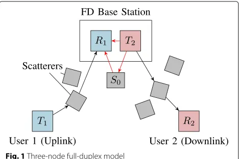
Currently deployed wireless communications equipment operates in half-duplex mode, meaning that transmis-sion and reception are orthogonalized either in time (time-division-duplex) or frequency (frequency-division-duplex). Research in recent years [1–12] has investigated the possibility of wireless equipment operating in full-duplex mode, meaning that the transceiver will both transmit and receive at the same time and in the same spectrum. A potential benefit of full-duplex is illustrated in. User 1 wishes to transmit uplink data to a base sta-tion, and User 2 wishes to receive downlink data from the same base station. If the base station is half-duplex, then it must either service the users in orthogonal time slots or in orthogonal frequency bands. However, if the base station can operate in full-duplex mode, then it can enhance spec-tral efficiency by servicing both users simultaneously. The challenge to full-duplex communication, however, is that the base station transmitter generates high-powered self-interference which potentially swamps its own receiver, precluding the detection of the uplink message.1

*Correspondence: [email protected]

This paper was presented in part at the 2014 IEEE International Symposium on Information Theory.

Department of Electrical and Computer Engineering, Rice University, Houston, TX 77005, USA

For full-duplex to be feasible, the self-interference must be suppressed. The two main approaches to self-interference suppression are cancellation and spatial isolation, and we now define each.Self-interference cancel-lationis any technique which exploits the foreknowledge of the transmit signal by subtracting an estimate of the self-interference from the received signal. Cancellation can be applied at digital baseband, at analog baseband, at RF, or, as is most common, applied at a combination of these three domains [4–7, 11, 13, 14]. Spatial isola-tionis any technique to spatially orthogonalize the self-interference and the signal-of-interest. Some spatial isola-tion techniques studied in the literature are multi-antenna beamforming [1, 15–19], directional antennas [20], shield-ing via absorptive materials [21], and cross-polarization of transmit and receive antennas [10, 21]. The key dif-ferentiator between cancellation and spatial isolation is that cancellation requires and exploits knowledge of the self-interference, while spatial isolation does not. To our knowledge, all full-duplex designs to date have required both cancellation and spatial isolation in order for full-duplex to be feasible even at very short ranges (i.e.,< 10 m). For example, see designs such as [5, 6, 10, 11], each of which leverages cancellation techniques as well as at least one spatial isolation technique. Moreover, because cancel-lation performance is limited by transceiver impairments such as phase noise [22], spatial isolation often accounts

for an outsized portion of the overall self-interference suppression.

For example, in the full-duplex design of [21] which demonstrated full-duplex feasibility at WiFi ranges, of the 95 dB of self-interference suppression achieved, 70 dB is due to spatial isolation, while only 25 dB is due to cancella-tion. Therefore, if full-duplex feasibility is to be extended from WiFi-typical ranges to the ranges typical of femto-cells or even larger femto-cells, then excellent spatial isolation performance will be required, hence our focus is on spatial isolation in this paper.

In a previous work [21], we studied three passive tech-niques for spatial isolation: directional antennas, absorp-tive shielding, and cross-polarization, and measured their performance in a prototype base station both in an ane-choic chamber that mimics free space, and in a reflec-tive room. As expected, the techniques suppressed the self-interference quite well (more than 70 dB) in an ane-choic chamber, but scattering environments, the sup-pression was much less, (no more than 45 dB), due to the fact that passive techniques operate primarily on the direct path between the transmit and receive antennas, and do little to suppress paths that include an external backscatterer. The direct-path limitation of passive spa-tial isolation mechanisms raises the question of whether or not spatial isolation can be useful in a backscatter-ing environment. Another class of spatial isolation tech-niques called “active” or “channel aware” spatial isolation [23] can indeed suppress both direct and backscattered self-interference. In particular, if multiple antennas are used and if the self-interference channel response can be estimated, then the radiation pattern can be shaped adaptively to mitigate both direct-path and backscat-tered self-interference. However, this pattern shaping (i.e., beamforming) will consume spatial degrees-of-freedom that could have otherwise been leveraged for spatial mul-tiplexing. Thus, there is an important tradeoff between spatial self-interference isolation and achievable degrees of freedom.

To appreciate the tradeoff, consider the example in Fig. 1. The direct path from the base station transmit-ter,T2, to its receiverR1, can be passively suppressed by

shielding the receiver from the transmitter as shown in [21], but there will also be backscattered self-interference due to objects near the base station (depicted by gray blocks in Fig. 1). The self-interference caused by scat-terer S0, for example, in Fig. 1, could be avoided by

creating a null in the direction of S0. However, losing

access to the scatterer could create a less-rich scattering environment, diminishing the spatial degrees-of-freedom of the uplink or downlink. Moreover, creating the null consumes spatial degrees-of-freedom that could other-wise be used for spatial multiplexing to the downlink user, diminishing the achievable degrees-of-freedom of

Fig. 1Three-node full-duplex model

the downlink. This example leads us to pose the following question.

Question: Under what scattering conditions can spatial isolation be leveraged in full-duplex operation to provide a degree-of-freedom gain over half-duplex? More specifi-cally, given a constraint on thesizeof the antenna arrays at the base station and at the user devices, and given a char-acterization of thespatial distributionof the scatterers in the environment, what is the uplink/downlink degree-of-freedom region when the only self-interference mitigation strategy is spatial isolation?

Modeling approach:To answer the above question, we leverage the antenna-theory-based channel model devel-oped by Poon, Broderson, and Tse in [24–26], which we will label the “PBT” model. In the PBT model, instead of constraining the number of antennas, thesize of the array is constrained. Furthermore, instead of considering a channel matrix drawn from a probability distribution, a channel transfer function which depends on the geo-metric position of the scatterers relative to the arrays is considered (Fig. 2).

Contribution:We extend the PBT model to the three-node full-duplex topology of Fig. 1, and derive the degree-of-freedom region, DFD: the set of all achievable

uplink/downlink degree-of-freedom tuples. By compar-ingDFDto DHD, the degree-of-freedom region achieved

by time-division half-duplex, we observe that full-duplex outperforms half-duplex, i.e.,DHD⊂DFD, in the following

two scenarios.

1. When the base station arrays are larger than the corresponding user arrays, the base station has a larger signal space than is needed for spatial multiplexing and can leverage the extra signal dimensions to form beams that avoid

self-interference (i.e., self-interference zero-forcing). 2. More interestingly, when the forward scattering

intervals and the backscattering intervals are not completely overlapped, the base station can avoid self-interference by signaling in the directions that scatter to the intended receiver, but do not backscatter to the base-station receiver. Moreover, the base station can also signal in directions thatdo cause self-interference, but ensure that the generated self-interference is incident on the base-station receiver only in directions in which uplink signal is not incident on the base-station receiver, i.e., signal such that the self-interference and uplink signal are spatially orthogonal.

In [27], an experimental evaluation of a transmit-beamforming-based method for full-duplex operation called “SoftNull” is presented. Inspired by the achievabil-ity proof in Section 3.1, the SoftNull algorithm presented in [27] seeks to maximally suppress self-interference for a given required number of downlink-degrees-of-freedom. This paper presents an information theoretic analysis of the performance limits of beamforming-based full-duplex systems, whereas [27] presents an experimental evalua-tion of a specific design. We would like to refer [27] to readers who may be interested in how the theoretical intuitions from this paper can guide the design and imple-mentation of a beamforming-based full-duplex system.

Organization of the paper: Section 2 specifies the system model: we begin with an overview of the PBT model in Section 2.1 and then in Section 2.2 apply the model to the scenario of a full-duplex base station with uplink and downlink flows. Section 3 gives the main analysis of the paper, the derivation of the degrees-of-freedom region. We start Section 3 by stating the theorem which characterizes the degrees-of-freedom region and then give the achievability and converse arguments in Sections 3.1 and 3.2, respectively. In Section 4, we assess the impact of the degrees-of-freedom result on the design and deployment of full-duplex base stations, and include

an application example, that shows how the results of this paper are used to guide the design of a full-duplex base station in [27]. We give concluding remarks in Section 5.

2 System model

We now give a brief overview of the PBT channel model presented in [24]. We then extend the PBT model to the case of the three-node full-duplex topology of Fig. 1, and define the required mathematical formalism that will ease the degrees-of-freedom analysis in the sequel.

2.1 Overview of the PBT model

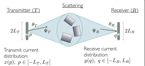
As illustrated in Fig. 3, the PBT channel model consid-ers a wireless communication link between a transmitter equipped with a unipolarized continuous linear array of length 2LT and a receiver with a similar array of length 2LR. The authors observe that there are two key domains: the array domain, which describes the current distribu-tion on the arrays, and the wavevector domain which describes radiated and received field patterns. Channel measurement campaigns show that the angles of depar-ture and the angles of arrival of the physical paths from a transmitter to a receiver tend to be concentrated within a handful of angular clusters [28–31]. Thus the authors of the PBT model [24] focus on the union of the clusters of angles-of-departure from the transmit array, denoted

T, and the union of the clusters of angles-of-arrival to the receive array, R. Because a linear array aligned to the z-axis array can only resolve the z-component, the intervals of interest are T = {cosθ : θ ∈ T} and R = {cosθ : θ ∈R}. In [24], it is shown from the first principles of Maxwell’s equations that an array of length 2LT has a resolution of 1/(2LT)over the intervalT, so that the dimension of the transmit signal space of radiated field patterns is 2LT|T|. Likewise the dimension of the receive signal space is 2LR|R|, so that the spatial degrees of freedom a point-to-point communication link,dP2P, is

dP2P=min{2LT|T|, 2LR|R|}. (1)

2.2 Extension of PBT model to three-node full-duplex

Now we extend the PBT channel model in [24], which considers a point-to-point topology, to the three-node full-duplex topology of Fig. 1. The antenna-theory-based PBT channel model is built upon far-field assumptions, i.e., that the propagation path is much larger than a wave-length. We acknowledge that direct-path self-interference may not obey far-field behavior. However, the backscat-tered self-interference, which will travel several wave-lengths to reach an external scatterer and then return to the base station, is indeed a far-field signal. As discussed in the introduction, the intent of this paper is to under-stand the impact of backscattered self-interference as a function of the size of antenna arrays and the geometric distribution of the scatterers. Since the backscattering is indeed a far-field phenomenon, the PBT model is a quite well-suited model for our study.

As in [24], we consider continuous linear arrays of infinitely many infinitesimally small unipolarized antenna elements.2 Each of the two transmitters Tj, j = 1, 2, is equipped with a linear array of length 2LTj, and each receiver, Ri, i = 1, 2, is equipped with a linear array of length 2LRi. The lengthsLTj and LRi are normalized by the wavelength of the carrier, and thus are unitless quantities. For each array, define a local coordinate sys-tem with origin at the midpoint of the array andz-axis aligned along the length of the array. Let θTj ∈[ 0,π ) denote the elevation angle relative to the Tj array, and letθRi denote the elevation angle relative to theRiarray. Denote the current distribution on theTjarray asxj(pj), where pj ∈[−LTj,LTj] is the position along the lengths of the array, and xj :[−LTj,LTj]→ C gives the magni-tude and phase of the current. The current distribution, xj(pj), is the transmit signal controlled by Tj, which we constrain to be square integrable. Likewise, we denote the received current distribution on theRiarray asyi(qi),qi∈ [−LRi,LRi].

The signal received by the base station receiver,R1, at a

pointq1∈[−LR2,LR2] along its array is given by

y1(q1)=

LT₁

−LT₁

C11(q1,p1)x1(p1)dp1

desired uplink signal

+

_LT

2

−LT₂

C12(q1,p2)x2(p2)dp2

self-interference

+z 1(q1), noise

(2)

where z1(q1), q1 ∈[−LR1,LR1] is the noise along theR1

array. The channel response integral kernel, Cij(qi,pj), gives the current excited at a pointqion the receive array due to a current at the point pj on the transmit array. Note that the first term in (2) gives the received uplink

signal-of-interest, while the second term gives the self-interference generated by the base station’s own transmis-sion. We assume that the mobile users are out of range of each other, such that there is no channel fromT1toR2.3

Thus,R2’s received signal at a pointq2∈[−LR2,LR2] is

y2(q2)=

LT₂

−LT₂

C22(q2,p2)x2(p2)dp2+z2(q2). (3)

The channel response kernel,Cij(·,·) is composed of a transmit array response, ATj(·,·), a scattering response, Hij(·,·), and a receive array response, ARi(·,·) [24]. The channel response kernel is given by

Cij(q,p)=

ARi(q,κˆ)

Rx array response

scattering response

Hij(κˆ,kˆ)

× ATj(kˆ,p)

Tx array response

dkˆdκˆ,

(4)

wherekˆ is a unit vector that gives the direction of depar-ture from the transmitter array, andκˆis a unit vector that gives the direction of arrival to the receiver array. The transmit array response kernel, ATj(kˆ,p), maps the cur-rent distribution along the Tj array (a function of p) to the field pattern radiated fromTj(a function of direction of departure,kˆ). The scattering response kernel,Hij(κˆ,kˆ), maps the fields radiated fromTjin directionkˆto the fields incident onRiat directionκˆ. The receive array response, ARi(q,κˆ), maps the field pattern incident onRi (a func-tion of direcfunc-tion of arrival,κˆ) to the current distribution excited on theRiarray (a function of positionq), which is the received signal.

2.3 Array responses

In [24], the transmit array response for a linear array is derived from the first principles of Maxwell’s equations and shown to be ATj(kˆ,p) = ATj(cosθTj,p) = e−i2πpcosθTj_,p∈−L

Tj,LTj

, whereθTj ∈[ 0,π )is the ele-vation angle relative to theTjarray. Due to the symmetry of the array (aligned to thez-axis), the radiation pattern is symmetric with respect to the azimuth angle and only depends on the elevation angle θ_Tj through cosθ_Tj. For notational convenience, lett ≡ cosθ_Tj ∈[−1, 1], so that we can simplify the transmit array response kernel to

ATj(t,p)=e−

i2πpt_{, t∈[−1, 1] , p∈−L} Tj,LTj

. (5)

By reciprocity, the receive array response kernel, ARi(q,κˆ), is

ARi(q,τ )=ei2

πqτ_{, τ ∈[−1, 1] ,q∈−L}

Ri,LRi

, (6)

and receive array response kernels are identical to the kernels of the Fourier transform and inverse Fourier trans-form, respectively, a relationship we will further explore in Section 2.5.

2.4 Scattering responses

The scattering response kernel,Hij(κˆ,kˆ), gives the ampli-tude and phase of the path departing fromTjat direction

ˆ

k and arriving atRi at directionκˆ. Since we are consid-ering linear arrays which only resolve the cosine of the elevation angle, we can considerHij(τ,t)which gives the superposition of the amplitude and phase of all paths ema-nating fromTj with an elevation angle whose cosine ist and arriving atRiat an elevation angle whose cosine isτ.

As is done in [24], motivated by measurements show-ing that scattershow-ing paths are clustered with respect to the transmitter and receiver, we adopt a model that focuses on theboundaryof the scattering clusters rather than the discrete paths themselves, as illustrated in Fig. 2.

Let(_Tk)

ijdenote the angle subtended at transmitterTjby thekth_{cluster that scatters toR}

i, and letTij = k

(k)

Tij be the total transmit scattering interval from Tj to Ri. This scattering interval,Tij, is the set of directions that when illuminated byTjscatters energy toRi. In Fig. 2, to avoid clutter, we illustrate the case in which(_Tk)

ij is a sin-gle contiguous angular interval, but in general, the interval will be non-contiguous and consist of several individual clusters. Similarly let(_Rk)

ij denote the corresponding angle subtended atRi by thekthcluster illuminated byTj, and letRij = k

(k)

Rij be set of directions from which energy can be incident onRifromTj.

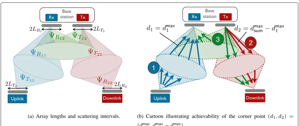
Thus, we see in Fig. 2 that from the point-of-view of the base-station transmitter,T2,T22is the angular

inter-val over which the base station can radiate signals that will reach the intended downlink receiver,R2. The

angu-lar interval,_T12, is the interval in which the base station’s radiated signals will backscatter to the base station’s own receiver,R1, as self-interference. Likewise, from the

point-of-view of the base station receiver,R1,R11, is the interval

over which the base station may receive signals from the uplink transmitter,T1, whileR12is the interval in which

self-interference may be present. Clearly, the extent to which the self-interference intervals and the signal-of-interest intervals overlap will have a major impact on the degrees of freedom of the network. Because linear arrays can only resolve the cosine of the elevation angle t ≡ cosθ, we define the “effective” scattering intervals for the transmit and receive arrays, respectively, as

Tij ≡

Define the size of the transmit and receive scattering intervals as|Tij| =

_Tijt dtand|Rij| =

_Rijτdτ.

As in [24], we assume the following characteristics of the scattering responses:

The first condition means that the scattering response is zero unless the angle of arrival and angle of departure both lie within their respective scattering intervals. The sec-ond csec-ondition means that in any direction of departure, t∈Tij, there exists at least one path from transmitterTj receiverRi. Similarly, the third condition implies that in any direction of arrival,τ ∈Rij, there exists at least one path fromTjtoRi. The fourth condition means that there are many paths from the transmitter to the receiver within the scattering intervals, so that the number of propagation paths that can be resolved within the scattering intervals is limited by the length of the arrays and not by the number of paths. The final condition aids our analysis by ensuring the corresponding integral operator is compact, but is also a physically justified assumption since one could argue for the stricter assumption₋1₁₋1₁|Hij(τ,t)|2dτdt ≤ 1, since no more energy can be scattered than is transmitted.

2.5 Hilbert space of wave-vectors

We can now write the original input-output relation given in (2) and (3) as

than current distributions over position along the array. In fact, for our case of the unipolarized linear array, the transmit and receive array responsesarethe Fourier and inverse-Fourier integral kernels, respectively.

LetTjbe the space of all field distributions that trans-mitter Tj’s array of length LTj can radiate towards the available scattering clusters, _Tjj ∪_Tij (both signal-of-interest and self-interference). In the vernacular of [24],Tj is the space of field distributions array-limited toLTj and wavevector-limited toTjj∪Tij. To be precise, defineTj to be the Hilbert space of all square-integrable functions Xj:Tjj∪Tij →C, that can be expressed as

Xj(t)= L_Tj

−L_Tj

ATj(t,p)xj(p)dp, t∈Tjj∪Tij

for somexj(p), p∈[−LTj,LTj]. The inner product defined for this Hilbert Space between two member functions, Uj,Vj ∈ Tj, is the usual inner product: Uj,Vj =

_Tjj∪_TijUj(t)Vj∗(t)dt. Likewise, let Ri be the space of field distributions that can be incident on receiverRifrom the available scattering clusters,Rii ∪Rij, and resolved by an array of lengthLRi. More precisely,Riis the Hilbert space of all square-integrable functionsYi :Rii∪Rij→ C, that can be expressed as

Yi(τ )= L_Ri

−L_Ri

A∗_Ri(q,τ )yi(q)dq, τ ∈Rii∪Rij

for some yi(q), q ∈[−LRi,LRi], with the same inner product. From [24], we know that the dimension of these array-limited and wavevector-limited transmit and receive spaces are, respectively,

dimTj=2LTj|Tjj∪Tij|, and (9) dimRi=2LRi|Rii∪Rij|. (10)

We can define the scattering integrals in (7) and (8) as operators mapping from one Hilbert space to another. Define the operatorHij:Tj→Riby

(HijXj)(τ )=

_Tij∪_Tjj

Hij(τ,t)Xj(t)dt, τ ∈Rij∪Rii.

(11)

We can now write the channel model of (7) and (8) in the wave-vector domain as

Y1=H11X1+H12X2+Z1, (12)

Y2=H22X2+Z2, (13)

whereXj∈Tj, forj=1, 2 andYi,Zi∈Rifori=1, 2. The following lemma states key properties of the scattering operators in (12–13) that we will leverage in our analysis.

Lemma 1The scattering operators Hij, (i,j) ∈ {(1, 1), (2, 2),(1, 2)}have the following properties:

1. The scattering operator,Hij:Tj→Ri, is a compact

operator.

2. The dimension of the range of the scattering operator,dimR(Hij)≡dimN(Hij)⊥, (i.e., the

dimension of the space orthogonal to the operator’s nullspace) is given by

dimR(Hij)=2 min{LTj|Tij|,LRi|Rij|}.

3. There exists a singular systemσ_ij(k),U_ij(k),V_ij(k)∞ k=1 for scattering operatorHij, where the singular value σ_ij(k)is nonzero if and only if

k≤2 min{LTj|Tij|,LRi|Rij|}.

Proof Property 1 holds because Hij(·,·), the kernel of integral operator Hij, is square integrable, and an inte-gral operator with a square integrable kernel is compact (see Theorem 8.8 of [32]). Property 2 is just a restate-ment of the main result of [24]. Property 3 follows from the first two properties: The compactness of Hij, estab-lished in Property 1, implies the existence of a singular system, since there exists a singular system for any com-pact operator (see Section 16.1 of [32]). Property 2 implies that only the first 2 min{LTj|Tij|,LRi|Rij|}of the singu-lar values will be nonzero, since theU_ij(k)corresponding to nonzero singular values form a basis forR(Hij), which has dimension 2 min{LTj|Tij|,LRi|Rij|}. See Lemma 5 in Appendix B for a description of the properties of singular systems for compact operators, or see Section 2.2 of [33] or Section 16.1 of [32] for a thorough treatment.

3 Spatial degrees-of-freedom analysis

We now give the main result of the paper: a characteriza-tion of the spatial degrees-of-freedom region for the PBT channel model applied to a full-duplex base station with uplink and downlink flows.

Theorem 1Let d1and d2, respectively, denote the

spa-tial degrees of freedom of the uplink data flow from T1

to R1, and the downlink data flow from T2 to R2. The

spatial degrees-of-freedom region,DFD, of the three-node

full-duplex channel is the convex hull of all spatial degrees-of-freedom tuples,(d1,d2), satisfying

d1≤dmax1 =2 min

LT1|T11|,LR1|R11|

, (14) d2≤dmax2 =2 min

LT2|T22|,LR2|R22|

, (15) d1+d2≤dsummax=2LT2|T22\T12| +2LR1|R11\R12|

+2 max(LT2|T12|,LR1|R12|). (16)

The degrees-of-freedom region characterized by Theorem 1, DFD, is the pentagon-shaped region shown

Fig. 4Degrees-of-freedom region,DFD

Theorem 1 is given in Section 3.1, and the converse is given in Section 3.2.

3.1 Achievability

Overview of achievability proof:Before launching into the full proof, we would like to give a brief sketch of the achievability of corner point (d₁,d₂) of the degrees-of-freedom regionDFDshown in Fig. 4. The steps for

achiev-ing the degrees-of-freedom tuple(d₁,d₂)=(dmax₁ ,dmax sum−

dmax₁ )are illustrated in Fig. 5b.

1. First, the uplink transmitter,T1, transmits the maximum number of data streams that the uplink channel will support,

dmax₁ =2 min(LT1|T11|,LR1|R11|)(illustrated by

blue arrows in Fig. 5b). The base station downlink

transmitter,T2, must then structure its transmit signal such that it does not interfere with the base station receiver’s reception of thesedmax₁ data streams, as is described in the following steps. 2. Second, the base station transmitter,T2, transmits as

many data streams as can be supported in the interval

T22\T12(illustrated by red arrows in Fig. 5b),

which is the interval over which signal will couple to the downlink userR2, but will not present any self-interference to the base station’s own receiverR1. 3. Third, the base station transmits as many data

streams as possible in the intervalT22∩T12while

ensuring that the self-interference is only incident on the base station receiver,R1over the interval

_R11\_R12(illustrated by green arrows in Fig. 5b), which is the interval over which no uplink signal

Fig. 5Diagrams illustrating the geometrical interpretation of the degrees-of-freedom regionDFDand the achievability strategy.aArray lengths and scattering intervals.bCartoon illustrating achievability of the corner point(d1,d2)=d1max,dmaxsum−dmax1

formT1will be incident on receiverR1. This step occupies a majority of the proof.

The final step in the achievability proof is to show that if the transmission strategies described in steps 1–3 are employed, that the receivers, R1 and R2, can

success-fully recover the d1- and d2-dimensional data streams,

respectively.

Full achievability proof:We establish achievability of

DFD by way of two lemmas. The first lemma shows the

achievability of two specific spatial degrees-of-freedom tuples, and the second shows that these tuples are indeed the corner points ofDFD.

Lemma 2 The spatial degree-of-freedom tuples(d₁,d₂) and(d₁,d₂), given below, are achievable:

d₁ =min2LT1|T11|, 2LR1|R11|

, (17)

d₂ =

mindT2, 2LR2|R22|

, LT1|T11| ≥LR1|R11|

minδT2, 2LR2|R22|

, otherwise , (18)

d₁=

min2LT1|T11|,dR1

, LR2|R22| ≥LT2|T22|

min2LT1|T11|,δR1

, otherwise , (19)

d₂=min2LT2|T22|, 2LR2|R22|

, (20)

where the terms dT2,δT2 dR1, andδR1 are given in(17–20)

within the table at the bottom of the page.

dT2=2LT2|T22\T12|

+2 minLT2|T22∩T12|,(LT2|T12|−LR1|R12|)+ +LR1|R12\R11|

(21)

δT2 =2LT2|T22\T12|

+2 minLT2|T22∩T12|,LT2|T12| −LT1|T11| −

LR1|R11\R12| +(LR1|R12| −LT2|T12|)+

(22)

dR1 =2LR1|R11\R12|

+2 minLR1|R11∩R12|,(LR1|R12|−LT2|T12|)+ +LT2|T12\T22|

(23)

δR1 =2LR1|R11\R12|

+2 min

LR1| R11∩R12|, LR1|R12| −

LR2|R22|

−LT2|T22\T12| +

LT2|T12|

−LR1|R12|

+

(24)

Proof Due to the symmetry of the problem, it suffices to demonstrate achievability of only the first spatial degree-of-freedom pair in Lemma 2, (d₁,d₂), as the second pair, (d₁,d₂), follows from symmetry. Thus we seek to prove the achievability of the tuple (d₁,d₂) given in (17-18). We will show achievability of (d₁,d₂) in the case where LT1|T11| ≥LR1|R11|, for which

d₁=2LR1|R11|, (25)

d₂=mindT2, 2LR2|R22|

, (26)

where

dT2=2LT2|T22\T12|

+min

2LT2|T22∩T12|,

2(LT2|T12| −LR1|R12|)++2LR1|R12\R11|

.

(27)

Achievability of (d₁,d₂) in the LT1|T11| < LR1|R11|

case is analogous.

We now begin the steps to show achievability of (25) and (26).

3.1.1 Defining key subspaces

We first define key subspaces of the transmit and receive wave-vector spaces (T1, T2, R1, and R2) that will be

crucial in demonstrating achievability.

Subspaces ofT2: Recall thatT2is the space of all field

distributions that can be radiated by the base station transmitter,T2, in the direction of the scatterer intervals,

T22∪T12, (both signal-of-interest and self-interference).

LetT22\12⊆T2be the subspace of field distributions that

can be transmitted byT2, which are nonzero only in the

interval_T22\_T12,

T22\12≡span

X2∈T2:X2(t)=0∀t∈T12

. (28)

More intuitively, T22\12 is the space of transmissions

from the base station which couple only to the intended downlink user, and do not couple back to the base station receiver as self-interference. Similarly letT12 ⊆ T2be the

subspace of functions that are only nonzero in the interval

_T12,

T12≡span

X2∈T2:X2(t)=0∀t∈/T12

, (29)

that is, the space of base station transmissions whichdo couple to the base station receiver as self-interference. Finally, letT22∩12 ⊆ T12 ⊆ T2 be the subspace of field

distributions that are nonzero only in the intervalT22∩ _T12,

T22∩12≡span{X2∈T2:X2(t)=0∀t∈/T22∩T12},

(30)

the result of [24], we know that the dimension of each of these transmit subspaces ofT1is as follows:

dimT12=2LT2|T12|, (31)

dimT22\12=2LT2|T22\T12|, (32)

dimT22∩12=2LT2|T22∩T12|. (33)

Definition 1We say that Hilbert spaceAis the orthog-onal direct sum of Hilbert spacesB andC if any a ∈ A can be decomposed as a = b+c , for some b ∈ Band c∈ C, where a and b are orthogonal. We use the notation A=B⊕Cto denote that A is the orthogonal direct sum of BandC.

One can check thatT12andT22\12are constructed such

that they form anorthogonal direct sumfor spaceT2:

T2=T12⊕T22\12, (34)

thus anyX2∈T2can be written asX2=X2Orth+X2Int, for

someX2Orth ∈ T22\12 andX2Int ∈ T12, such thatX2Orth ⊥

X2Int. By the construction ofT22\12,H12X2Orth = 0, since

H12(τ,t) = 0 ∀t ∈/ T12 and X2Orth ∈ T22\12 implies

X2Orth(t)=0∀t∈T12. In other words,X2Orth ∈T22\12is

zero everywhere the integral kernelH12(τ,t) is nonzero.

Thus, any transmitted field distribution that lies in the subspaceT22\12will not present any interference toR2.

Subspaces ofT1: Recall thatT1is the space of all field

distributions that can be radiated by the uplink user trans-mitter,T1, towards the available scatterers. LetT11 ⊆ T1

be the subspace of field distributions that can be transmit-ted byT1’s continuous linear array of lengthLT1which are

nonzero only in the interval_T11, more precisely

T11≡span{X1∈T1:X1(t)=0∀t∈/T11}. (35)

More intuitively,T11is the space of transmissions from

the uplink user which will couple to the base station receiver. From the result of [24], we know that

dimT11=2LT1|T11|. (36)

Note thatT11 = T1, since we have assumedT21 = ∅.

AlthoughT11is thus redundant, we define it for notational

consistency.

Subspaces ofR1: Recall thatR1is the space of all

inci-dent field distributions that can be resolved by the base station receiver, R1. Let R12 ⊆ R1 to be the subspace

of received field distributions which are nonzero only for

τ ∈_R12, that is

R12≡spanY1∈R1:Y1(τ )=0∀τ /∈R12

. (37)

Less formally,R12is the space of receptions at the base

station which could have emanated from the base stations own transmitter. Similarly, letR12\11 ⊆ R12 ⊆ R1 be

the subspace of received field distributions that are only nonzero forτ ∈R12\R11,

R12\11≡span

Y1∈R1:Y1(τ )=0∀τ ∈R11

.

(38)

Less formally, R12\11 is the space of receptions at the

base station which could have emanated from the base sta-tion transmitter, but could not have emanated from the uplink user. Finally, defineR11 ⊆ R1to be the subspace

of received field distributions that are nonzero only for

τ ∈_R11,

R11≡spanY1∈R1:Y1(τ )=0∀τ /∈R11

, (39)

the space of base station receptions which could have emanated from the intended uplink user. Note thatR1=

R11⊕R12\11. From the result of [24], we know the

dimen-sion of each of the above base-station receive subspaces is as follows:

dimR11=2LR1|R11|, (40)

dimR12\11=2LR1|R12\R11|, (41)

dimR12=2LR1|R12|. (42)

Subspaces of R2: Recall that R2 is the space of all

incident field distributions that can be resolved by the downlink user receiver,R2. LetR22 ⊆ R2to be the

sub-space of received field distributions which are nonzero only forτ ∈_R22, that is

R22≡span

Y2∈R2:Y2(τ )=0∀τ /∈R22

. (43)

Note thatR22= R2, since we have assumedR21 = ∅.

AlthoughR22 is thus redundant, we define it for

nota-tional consistency. By substituting the subspace dimen-sions given above into (25) and (27), we can restate the degree-of-freedom pair whose achievability we are estab-lishing as

d₁,d₂=dimR11, min

dT2, dimR22 , where

(44)

dT2 =dimT22\12 +min

dimT22∩12,

(dimT12−dimR12)++dimR12\11

.

(45)

Now that we have defined the relevant subspaces, we can show how these subspaces are leveraged in the trans-mission and reception scheme that achieves the spatial degrees-of-freedom tuple(d₁,d₂).

3.1.2 Spatial processing at each transmitter/receiver

Processing at uplink user transmitter,T1:Recall that

d₁ = dimR11 is the number of spatial

degrees-of-freedom we wish to achieve for Flow1, the uplink flow.

Let χ₁(k) d₁

k=1, χ

(i)

1 ∈ C, be the d1 symbols that T1

wishes to transmit to R1. We know from Lemma 1 that

there exists a singular value expansion for H11, so let

σ₁₁(k),U₁₁(k),V₁₁(k) ∞

k=1be a singular system for the

opera-torH11 : T1 →R1(see Lemma 5 in Appendix B for the

definition of a singular system).

Note that the functionsV₁₁(k)dimT1

k=1 form an

orthonor-mal basis for T1, and since d1 = dimR11 ≤ dimT1,

there are at least as many such basis functions as there are symbols to transmit.

We constructX1, the transmit wave-vector signal

trans-mitted byT1, as

Processing at the base station transmitter,T2:

Recall that d₂ = mindT2, 2LR2|R22|

, wheredT2 is

given in (27), is the number of spatial degrees-of-freedom we wish to achieve for Flow2, the downlink flow. Let

χ₂(k)

d₂

k=1 be thed

2symbols that T2 wishes to transmit

toR2. We split theT2transmit signal into the sum of two

orthogonal components,X2Orth ∈ T22\12andX2Int ∈ T12,

so that the wave-vector signal transmitted byT2is

X2=X2Orth+X2Int, X2Orth∈T22\12, X2Int ∈T12.

orthonormal basis forT22\12, and let

d_2Orth≡mindimT22\12, dimR22

, (48)

be the number of symbols that T2 will transmit along

X2Orth. We constructX2Orthas

Recall that there ared₂total symbols thatT2wishes to

transmit, and we have transmitted d₂

Orth symbols along

X2Orth, thus there are d2 − d2Orth symbols remaining to

transmit alongX2Int. Let

d_2Int ≡d₂−d₂

X2Int will present interference toR1. Therefore, we must

constructX2Intsuch that it communicatesd2Intsymbols to

R2, without impedingR1from recovering thed1symbols

transmitted fromT1. Thus, the construction ofX2Int ∈T12

will indeed depend on the structure ofH12.

First consider the case where dimT12 ≤ dimR12. In

this case, Eq. (50), which gives the number of symbols that must be transmitted alongX2Int, simplifies tod2Int =

mindimT22∩12, dimR12\11,(dimR22−dimT22\12)+

of dimT12≤dimR12(the case for which are constructing

X2Int), we have symbols to transmit alongX2Int. We constructX2Intas

X2Int=

Now we will consider the construction ofX2Int for the

other case where dimT12 > dimR12. In the dimT12 >

dimR12case Eq. (50), which gives the number of symbols

that must be transmitted alongX2Int, simplifies to

d_2Int =min

Note that the signal that R1 receives from T1 will

lie only in R11. Thus, if we can ensure that the

sig-nal from T2 falls in the orthogonal space, R12\11, then

we have avoided interference. Let H₁₂ : T12 → R12

be the restriction of H12 : T2 → R1 to domain

T12 and codomain R12. We consider the constriction, H₁₂, instead of H12 so that the preimage under H₁₂

is a subset of T12, so that any functions within this

not be interfered overτ ∈ R11 asH12 X2Int ∈ R12\11, or

equivalentlyX2Int ∈P12\11, where

P12\11≡H12←(R12\11)⊆T12, (54)

is the preimage ofR12\11underH₁₂. Thus, any function in

P12\11can be used for signaling toR2without interfering

X1atR1. The number of symbols that can be transmitted

will thus depend on the dimension of this interference-free preimage. Corollary 1 in the appendix states that if

C:X →Yis a linear operator with closed range, andSis finite dimensional subspace of a normed space is closed, R(H₁₂)is closed. Further, note that since we are consid-ering the case where dimT12 > dimR12, it is easy to see

thatR(H₁₂)=R12, which impliesR12\11 ⊆R(H₁₂), since

R12\11 ⊆R12by construction. Thus, the linear operator H₁₂ :T12→R12and the subspaceR12\11satisfy the

con-ditions on operatorCand subspaceS, respectively, in the hypothesis of Corollary 1. Thus, we can apply Corollary 1 to show that, when dimT12 > dimR12, the dimension of

Therefore, the dimension of P12\11, the preimage of

R12\11 underH₁₂, is indeed large enough to allowT2to

transmit the remainingd₂

Intsymbols along the basis

func-tions of dimP12\11. Let

In summary, combining all cases we see that the wavevector transmitted byT2is

X2=X2Orth+X2Int=

Now that we have constructedX1, the uplink

wavevec-tor signal transmitted on the the uplink user, andX2, the

wavevector signal transmitted on the dowlink by the base station, we show how the base station receiver,R1and the

downlink userR2process their received signals to detect

the original information-bearing symbols.

Processing at the base station receiver,R1:We need

to show thatR1can obtain at leastd1=dimR11

indepen-dent linear combinations of thed₁ symbols transmitted fromT1, and that each of these linear combinations are

corrupted only by noise, and not interference fromT2.

In the case where dimT12 > dimR12, T2 constructed

X2such thatH12X2is orthogonal to any function inR11.

Therefore,R1can eliminate interference fromT2by

sim-ply projectingY1ontoR11to recover the dimR11 linear

combinations it needs. We now formalize this projection ontoR11. Recall that the set of left-singular functions of

H11,

structs the set of complex scalars

. One can check that result of each of these projections is

nations of the intended symbols corrupted only by noise, as desired. Moreover, in this case the obtained linear combinations are already diagonalized, with thelth pro-jection only containing a contribution from thelth desired symbol.

In the case where dimT12 ≤ dimR12,H12X2in general

will not be orthogonal to every function inR11, and some

First, R1 can recover dimR11\12 interference-free linear

combinations by projecting its received signal, Y1, onto

R11\12. Let

J₁₁(l)_\12

dimR11\12

l=1 be an orthonormal basis for

R11\12. ReceiverR1forms a set of complex scalars

Therefore, eachξ₁(l) will be interference free, i.e., will be a linear combination of the symbolsχ₁(l)

bols. One can check that these dimR11\12 projections

result in

interference-free linear combinations of T1’s symbols so

that R1 can solve the system and recover the symbols.

Receiver R1 will obtain these linear combinations via a

careful projection onto a subspace ofR12 (which is the

orthogonal complement ofR11\12, the space onto which

we have already projectedY1to obtain the first dimR11\12

linear combinations). Recall that the set of left-singular

functions ofH12,

U₁₂(l)

dimR12

l=1 , form an orthonormal basis

forR12. ReceiverR1obtains the remainingR11∩12linear

combinations by projectingY1onto the last dimR11∩12

of these basis functions, forming

We compute the terms of Eq. (64) individually. The contribution ofT1’s transmit wavevector is

"

In the first step, (65), we use the singular function decomposition ofH11. In the second step, (66), we plug

in the construction ofX1given in 46, and in the last step,

(67), we leverage the fact that&_iχ₁(i) "

V₁₁(m),V₁₁(i)#=χ₁(m), due to the orthonormality of the right singular functions. The contribution ofT2’s interfering wavevector is

In step (68) above, we use the fact thatH12X2Orth = 0

by the construction ofX2Orth. Step (69) uses the singular

function expansion ofH12, step (70) substitutes the

con-struction ofX2Int, step (71) rearranges terms and step (72)

leverages the orthonormality of the right singular func-tions. In the last step, (74), we have leveraged that when dimT12≤dimR12,d2Int≤dimR12\11(see Eq. 50), which

means the largest value of i in the summation, d_2Int, is smaller that the smallest value of dimR12−kunder

con-sideration, dimR12−R11∩12+1 = dimR12\11+1, so

that the delta-functionδ(i,dimR12−k)will never evaluate to

one. Substituting (67) and (74) back into (64) shows that the output symbols obtained by projectingY1onto the last

R11∩12functions of

Combining the processing in all cases, we see that receiver R1 has formed a set of d1 complex scalars

Thus, as desired, in all cases the base station receiver R1is able to obtaind1interference-free linear

combina-tions of thed₁ symbols from the uplink user transmitter T1. Now, we move to the processing at the downlink user

receiver.

Processing at R2: We wish to show that the

down-link receiver,R2, can recover thed₂symbols transmitted

by the base station transmitter,Tw. Let

σ₂₂(k),U₂₂(k),V₂₂(k)

be a singular system for the operator H22, and let

r22 ≡ min2LT2|T22|, 2LR2|R22|

. From Property 2 of

Lemma 1, we know thatσ₂₂(k)is zero for allk > r22 and

3.1.3 Reducing to parallel point-to-point vector channels

The above processing at each transmitter and receiver has allowed the receiversR1andR2to recover the symbols

ξ₁(l)= respectively, where the linear combination coefficients, a(₁lm)anda(₂lm), are given in (77) and (81), respectively, and the additive noise on each of the recovered symbols,ζ₁(l)

andζ₂(l), are given in (78) and (82), respectively. We can rewrite (83-84) in matrix notation as

ξ₁=A1χ1+ζ1, (85)

ξ₂=A2χ2+ζ2, (86)

where χ₁ andχ₂ are thed₁ × 1 andd₂×1 vectors of input symbols for transmitters T1 and T2, respectively, ζ₁ andζ₂are thed₁×1 andd₂ ×1 vectors of additive noise, respectively, andA1andA2ared1×d1andd2×d2

square matrices whose elements are taken froma(₁lm)and a(₂lm), respectively. The matrices A1 andA2 will be full

rank for all but a measure-zero set of channel response kernels. Also, since each of theζ_j(l)’s are linear combina-tions of Gaussian random variables, the the noise vectors,

processing has reduced the original channel to two paral-lel full-rank Gaussian vector channels: the first ad₁ ×d₁ channel and the second ad₂×d₂channel, which are well known to have d₁ and d₂ degrees-of-freedom, respec-tively [34]. Therefore, the spatial degrees-of-freedom pair

(d₁,d₂)is indeed achievable.

Lemma 3The degree-of-freedom pairs (d₁,d₂) and (d₁,d₂), are the corner points ofDFD, that is

(d₁,d₂)=dmax₁ , mind₂max,dmax_sum−dmax₁ (87)

(d₁,d₂)=mindmax₁ ,dsummax−dmax2

,dmax₂ . (88)

ProofNote that it is sufficient to prove only Eq. (87), as Eq. (88) follows by the symmetry of the expressions. It is easy to see that d₁ = min

2LT1|T11|, 2LR1|R11|

= dmax₁ , but it is not so obvious that d₂ = mindmax₂ ,dmax

sum−d1max

. However, one can verify that d₂ = min{dmax₂ ,dmax

sum −dmax1 } by evaluating

the left- and right-hand sides for all combinations of the conditions

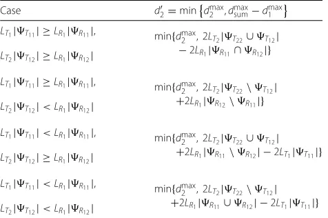
LT1|T11|LR1|R11|, (89)

LT2|T12|LR1|R12| (90)

and observing equality in each of the four cases. Table 1 shows the expressions to which d₂ and mindmax₂ ,dmaxsum−d1max

both simplify in each of the four possible cases.

Lemmas 2 and 3 show that the corner points of DFD, (d₁,d₂) and(d₁,d₂) are achievable. And, thus, all other points withinDFDare achievable via time sharing between

the schemes that achieve the corner points.

3.2 Converse

To establish the converse part of Theorem 1, we must show that the regionDFD, which we have already shown

Table 1Verifying that the corner points of inner and outer bounds coincide

Case d₂=mindmax

2 ,dmaxsum−dmax1

LT1|T11| ≥LR1|R11|, _min{_dmax

2 , 2LT2|T22∪T12| −2LR1|R11∩R12|}

LT2|T12| ≥LR1|R12|

LT1|T11| ≥LR1|R11|, _min{_dmax

2 , 2LT2|T22\T12| +2LR1|R12\R11|}

LT2|T12|<LR1|R12|

LT1|T11|<LR1|R11|, _min{_dmax

2 , 2LT2|T22∪T12| +2LR1|R11\R12| −2LT1|T11|}

LT2|T12| ≥LR1|R12|

LT1|T11|<LR1|R11|, _min{_dmax

2 , 2LT2|T22\T12| +2LR1|R11∪R12| −2LT1|T11|}

LT2|T12|<LR1|R12|

is achievable, is also an outer bound on the degrees-of-freedom, i.e., we want to show that if an arbitrary degree-of-freedom pair(d1,d2)is achievable, then(d1,d2)∈DFD.

It is easy to see that if (d1,d2) is achievable, then the

singe-user constraints on DFD, given in (14) and (15),

must be satisfied as the degrees-of-freedom for each flow cannot be more than the point-to-point degrees-of-freedom shown in [24]. Thus, the only step remaining in the converse is to establish an outer bound on the sum degrees-of-freedom which coincides withdmaxsum, the

sum-degrees-of-freedom constraint on the achievable region,

DFD, given in (16).

Thus, to conclude the converse argument, we will now prove the following Genie-aided outer bound on the sum degrees-of-freedom which coincides with the sum-degrees-of-freedom constraint on the achievable region.

Lemma 4

d1+d2≤ dmaxsum=2LT2|T22\T12| +2LR1|R11\R12| +2 max(LT2|T12|,LR1|R12|).

(91)

Sketch of proof: Before diving into the full proof, we would first like to give a brief overview of the steps in the converse proof. Our process for proving Lemma 4 is twofold.

1) First, a genie expands the transmit scattering intervalsT22andT12until the two intervals are

fully overlapped, and likewise expands expandsR11

andR12until they are fully overlapped, as shown in

Fig. 6. To ensure that the net manipulation of the genie can only enlargeDFD, the genie also increases

the array lengthsLT2 andLR1 sufficiently for any

added interference due to the expansion of_T12and

R12to be compensated by the increased array

lengths.

2) After the above genie manipulation is performed, the

maximum of theT2andR1signaling dimensions are

equal todmax_sumin constraint (16), and since the scattering intervals are overlapped, the channel model becomes the Hilbert space equivalent of the

well-studied MIMOZ -channel [35, 36]. The Hilbert

space analog to the bounding techniques employed in [35, 36] are then leveraged to conclude the converse proof.

ProofWe prove Lemma 4 by way of a Genie that aids the transmitters and receivers by enlarging the scattering intervals and lengthening the antenna arrays in a way that can only enlarge the degrees-of-freedom region. Applying the point-to-point bounds to the Genie-aided system in a careful way then establishes the outer bound. Assume an arbitrary scheme achieves the degrees-of-freedom pair

(d1,d2). Thus receiversR1andR2can decode their

corre-sponding messages with probability of error approaching zero. We must show that the assumption of(d1,d2)being

achievable implies the constraint in Eq. (91).

Let a Genie expand both scattering intervals atT2into

the union of the two scattering intervals, that is expand

T22andT12to

_T22=_T12=_T2 ≡T22∪T12.

Likewise, the Genie expands the scattering intervals at R1into their union, that is expandR11andR12to

_R

11 =

R12≡

R1 =R11∪R12.

The Genie’s expansion ofT22toT2 can only enlarge

the degrees-of-freedom region, as T2 could simply not

transmit in the added interval_T

2\T22(i.e., ignore the

added dimensions for signaling toR2) to obtain the

orig-inal scenario. Likewise, expandingR11 toR1 will only

enlarge the degrees-of-freedom region asR1 can ignore

the portion of the wavevector received over_R 1 \R11

to obtain the original scenario. However, expanding the interference scattering clusters, _T12 and _R12, to _T

2

and_R

1, respectively, can indeed shrink the

degrees-of-freedom region due to the additional interference caused by the added overlap with the signal-of-interest intervals

T22andR22, respectively. We need a final Genie

manip-ulation to compensate for this added interference, so that the net Genie manipulation can only enlarge the degrees-of-freedom region. Therefore, in the next step we will have the Genie lengthen the arrays at T2 and R1

suffi-ciently to allow any interference introduced by expanding

_T12 and_R12, to_T

2 and

R1, respectively, to be

zero-forced without sacrificing any previously available degrees of freedom. Expansion of T12 to T2 ≡ T22 ∪T12

causes the dimension of the interference thatT2presents

to R1 to increase by at most 2LT2|T22 \ T12|.

There-fore, let the Genie also lengthenR1’s array from 2LR1 to

2LR1 =2LR1 +2LT2

|T₂₂\T₁₂|

|R₁₁∪R₁₂|, so that the dimension of the total receive space at R1, dimR1, is increased from

dimR1=2LR1|R11∪R12|to

dimR₁=2LR1|R11∪R12| (92) =

'

2LR1+2LT2

|T22\T12| |R11∪R12|

(

|_R11∪_R12|

(93)

=2LR1|R11∪R12| +2LT2|T22\T12|

(94)

=dimR1+2LT2|T22\T12|. (95)

We observe in (95), that the Genie’s lengthening of the T2array by 2LT2

|T₂₂\T₁₂|

|R₁₁∪R₁₂| has increased the dimension of R1’s total receive signal space by 2LT2|T22 \ T12|,

which is the worst case increase in the dimension of the interference from T2 due to expansion of T12 to T22∪T12. Therefore, the dimension of the subspace of R

1which is orthogonal to the interference fromT2 will

be at least as large as in the original orthogonal space of R1. Thus, the combined expansion of T12 to T2

and lengthening of theR1array toLR1 can only enlarge

the degrees-of-freedom region. Analogously, expansion of

R12 to R1 ≡ R11 ∪R12 increases the dimension of R12, the subspace ofR1’s receive space which is

vulnera-ble to interference fromT2, by at most 2LR1|R11\R12|.

Therefore, let the Genie lengthen T2’s array from 2LT2

to 2LT2 = 2LT2 + 2LR1

|R₁₁\R₁₂|

|T₂₂∪T₁₂|, so that the dimen-sion of the transmit space atT2, dimT2, is increased from

dimT2=2LT2|T22∪T12|to

dimT₂=2LT2|T22∪T12| (96) =

'

2LT2+2LR1

|_R11\_R12| |T22∪T12|

(

|T22∪T12|

(97)

=2LT2|T22∪T12| +2LR1|R11\R12| (98) =dimT2+2LR1|R11\R12|. (99)

We see in (99) that the Genie’s lengthening ofT2’s array

to 2LT2 increases the dimension of T2’s transmit signal

space by 2LR1|R11\R12|, which is the worst case increase

in the dimension of the subspace ofR1’s receive subspace

vulnerable to interference from T2. Therefore, T1 can

leverage these extra 2LR1|R11\R12|dimensions to zero

force to the subspace ofR1’s receive space that has become

vulnerable to interference fromT2due to the expansion

R12toR1. Thus, the net effect of the Genie’s expansion

ofT2’s interference scattering interval,R12, toR1 and

lengthening of theT2array to 2LT2 can only enlarge the

The Genie-aided channel is illustrated in Fig. 6, which emphasizes the fact that the Genie has made the chan-nelfully-coupled in the sense that the signal-of-interest scattering and the interference scattering intervals are identical: any direction of departure fromT2which

scat-ters toR2also scatters toR1, and any direction of arrival

toR1which signal can be received fromT1is a direction

from which signal can be received fromT2. Note that for

the Genie-aided channel,

which is the outer bound on sum degrees-of-freedom that we wish to prove. Thus, if we can show that for the Genie-aided channel then the converse is established. Because the Genie-aided channel is now fully coupled, it is similar to the continuous Hilbert space analog of the full-rank discrete-antennas MIMOZinterference channel. Thus, the remaining steps in the converse argument are inspired by the techniques used in [35–37] for outer bounding the degrees-of-freedom of the MIMO interference channel.

Consider the case in which dimT₂≤dimR₁. Since our Genie has enforced_T

22 =

T12 and we have assumed

dimT₂ ≤ dimR₁, receiverR1 has access to the entire

signal space ofT2, i.e.,T2cannot zero force toR1.

More-over, by our hypothesis that(d1,d2) is achieved,R1can

decode the message from T1, and can thus reconstruct

and subtract the signal received fromT1from its received

signal.

SinceR1has access to the entire signal-space ofT2, after

removing the signal fromT1the only barrier to R1 also

decoding the message fromT2is the receiver noise

pro-cess. If it is not already the case, let a Genie lower the noise at receiverR1untilT2has a better channel toR1thanR2

(this can only increase the capacity region sinceR1could

always locally generate and add noise to obtain the orig-inal channel statistics). By hypothesis,R2can decode the

message fromT2, and sinceT2has a better channel toR1

thanR2,R1can also decode the message fromT1.

Since R1 can decode the messages from both T1 and

T2, we can bound the degrees-of-freedom region of the

Genie-aided channel by the corresponding point-to-point channel in whichT1andT2cooperate to jointly

communi-cate their messages toR1, which has degrees-of-freedom

mindimT₁+dimT₂, dimR₁, which implies that d1+d2≤dimR1, when dimT2≤dimR1. (108)

Now, consider the alternate case in which dimT₂ <

dimR₁. In this case, we let a Genie increase the length

access to the entire transmit signal space ofT2, we can use

the same argument we leveraged above in the dimT₂ ≤ dimR₁case to show that

d1+d2≤dimR1=dimT2, when dimT2>dimR1.

(111)

Combining the bounds in (108) and (111) yields,

d1+d2≤ max(dimT2, dimR1)