R E S E A R C H
Open Access
Analysis and experimental evaluation of the
frequency response of an indoor radiating cable
in the UHF band
Jorge A Seseña-Osorio
1*, Ignacio E Zaldívar-Huerta
1, Alejandro Aragón-Zavala
2and Gerardo A Castañón-Ávila
3Abstract
We present the modeling of the frequency response of the channel for a radiating cable system by using an autoregressive model for an indoor environment. The coefficients of the autoregressive model are determined from the experimental channel frequency response. Measurements were carried out in an indoor environment, in particular on the second floor of a university building in the frequency range of 1.3 to 1.8 GHz by using a vector network analyzer. It is demonstrated that the use of a second-order model provides a better representation of the behavior of the channel. In this context, the coherence bandwidth and thermsdelay spread show dependence with the receiver position along the radiating cable length. This dependence is crucial and must be taken into account in the design and study of broadband systems with mobility because thermsdelay spread and coherence bandwidth are used to describe the time dispersion and the frequency selectivity of the multipath fading channels, respectively.
Keywords:Radiating cable; Indoor propagation; Wireless communications; Channel modeling; Autoregressive processes
1 Introduction
The improvement in wireless technology systems and devices has contributed to a greater concentration of mobile devices in specific locations as well as an increase in the data transmission rate. Consequently, wireless service providers and researchers are becoming more interested in obtaining the best possible performance of wireless systems under such conditions. In this context, radiating cables have been used as alternative distributed antenna systems in order to obtain optimal coverage levels in any underground or closed environment [1-4]. However, it is well-known that, for indoor wireless communications, constructive and destructive interferences have a crucial effect on the signal being transmitted. Therefore, knowledge of the behavior of the wireless channel is essential for planning and studying of any wireless systems.
A radiating cable or leaky feeder is a coaxial cable where the outer conductor has been slotted, allowing radiation to occur along the cable length for uniform coverage. Thus, radiating cables are used to distribute radio waves
in sites where common antennas fail, besides being used as part of wireless systems such as radio detection systems and wireless indoor-positioning systems [5,6]. In recent years, the use of radiating cables has increased especially to provide cellular coverage in train and underground stations for which either macrocell penetration or an indoor distributed antenna system is not suitable. The coverage footprint provided by a radiating cable can normally be better shaped, thus filling in coverage holes in specific corridor scenarios much better than antennas and better containing leakage [3]. As prices are coming down in the manufacturing and installation of radiating cables, indoor radio solutions that include radiating cable are thus a very viable alternative nowadays. However, as stated in [3], antennas are more suitable to provide coverage in areas where the installation of radiating cables is much harder or unfeasible. On the other hand, the installation of radiating cables is a more sophisti-cated procedure and more costly than that of antenna installation. If coverage is to be focused on a specific area, the radiation characteristics of directional antennas can be utilized to maximize such coverage in the desired location, something that is much harder to achieve with the use of radiating cables. In summary, although radiating * Correspondence:[email protected]
1
Instituto Nacional de Astrofísica Óptica y Electrónica (INAOE), Calle Luis Enrique Erro No. 1, Tonantzintla, Puebla C.P. 72840, Mexico
Full list of author information is available at the end of the article
cables are a good alternative for some specific indoor envi-ronments such as corridors, there are other instances where antennas still are the preferred choice.
In order to accurately estimate the coverage and ex-pected data rate that could be obtained using a radiating cable system, channel modeling needs to be performed. Narrowband modeling will allow engineers and designers to estimate local mean coverage if the radiating cable is installed in a venue. This issue is particularly important for voice systems, where full received signal strength and signal-to-interference and noise ratio (SINR) are import-ant parameters that affect the performance of the system. However, if broadband data communications are to be deployed, it is very important that wideband channel characteristics be modeled, and hence, the maximum achievable data rate can be determined. Herein lies the main focus of this paper.
In [7], a typical narrowband propagation model for radiating cable systems is reported which takes into account the coupling and longitudinal losses of the radiating cable. At the same time, the slow and fast variations of the received signal levels are modeled by a log-normal distribution and a Rayleigh or Rician distribu-tion, respectively. In the case of the signal being consid-ered as a narrowband signal, such mentioned propagation models could be sufficient to design and study a radiating cable system. However, if a digital communication is being considered with high speed of data transmission, it is
necessary to study the frequency response and the rms
delay spread of the channel. In this context, little attention has been paid to such issues in radiating cable systems.
For example, in [7] and [8], only the rms delay spread
values have been reported and not it’s modeling. The fre-quency response modeling allows classifying the channel as frequency selective or flat fading channel by calculating the coherence bandwidth, and thermsdelay spread allows knowing the limits of the transmission rate. This fact is very important in most modern technologies because such technologies require wide bandwidths and high-transmission rate. In summary, a wideband propagation model allows knowing some system characteristics, for example, the frequency selectivity, intersymbol interfer-ence, and error floor.
The modeling of wideband channel can be developed by using time-domain or frequency-domain measurements, where the direct measurement of the impulse response or the frequency response of the channel is carried out, respectively. Time-domain measurement methods require various parameters to describe wideband channels but do not provide information of the signal phase. In contrast, using a frequency-domain measurement system, the mag-nitude and phase of the signal are known. Furthermore, an autoregressive model can be used to represent the channel with fewer parameters than in the case of
time-domain measurements. For indoor measurements, the frequency-domain approach yields very good results, having limited applicability for outdoor measurements since the coax cable length is a strong limitation for this.
To the best of the authors' knowledge, we report for the first time the autoregressive modeling of the frequency response of channel for a radiating cable system, as well as the rms delay spread (τrms) which showed a dependency with the receiver position along the cable length. Autore-gressive (AR) models in the frequency domain for indoor radio propagation have been reported in different studies [9,10]; however, such studies were based on wireless systems where the receiver and transmitter used conven-tional antennas. In contrast, the results of this work are for a wireless system which uses a radiating cable. Results showed that a second order of the autoregressive model gave the best fit to the complementary cumulative distri-bution of the coherence bandwidth (the 3-dB width of the frequency correlation function) and showed a better description of the signal delay.
The paper is organized as follows: Section 2 gives the methodology used in this study as well as the general description of the measurements and the autoregressive modeling of the channel frequency response. Section 3 is devoted to the analysis of results along with a brief discussion about the importance of the dependency of
rms delay spread with the receiver position along the
cable length. Finally, conclusions are given in Section 4.
2 Methodology, description of measurements, and the frequency-domain channel modeling 2.1 Methodology
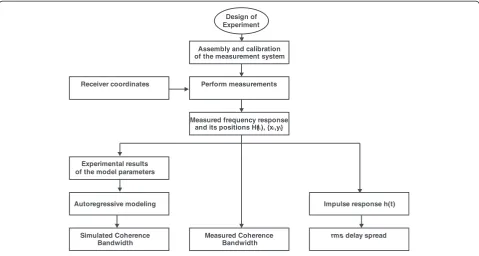
In order to model the frequency response of the chan-nel, the methodology developed in this study is depicted in Figure 1. The comparison of results is carried out by calculating the coherence bandwidth of the channel. At
the same time, the rms delay spread was calculated in
order to understand the relation between model parame-ters and the signal delay in the channel. A brief method-ology description is given below.
frequency responses and coherence bandwidth were calculated.
The complex frequency response of the channel is given by [11]:
H fð Þ ¼XL
i¼1βiexpð−j2πfτiÞexpð−jφiÞ ð1Þ
where βi, τi, and ϕi represent the magnitude, arrival
time, and phase, respectively, of the L individual paths
between the transmitter and receiver. Meanwhile, the channel is considered slowly time-varying. In practice, the response frequency of the channel can be measured by using a network analyzer, which sweeps the channel at discrete frequencies and measures the complex sam-ples of the frequency response. Thus, the samsam-ples of the complex frequency response of the channel is given by:
H kð Þ ¼H fk jfk¼kΔf ¼X
where N is the number of complex samples of the
fre-quency response andΔfis the frequency sample spacing.
If it is assumed thatf0= 0, then Equation2is the baseband
complex frequency response of the channel. Because the measurement system is band limited, the system measures
windowed frequency characteristics of the channel. There-fore, the measured frequency response is given as:
Hmeasð Þ ¼k W kð Þ
XL
i¼1βiexpð−j2πkΔfτiÞexpð−jφiÞ; 0≤k<N
ð3Þ
where W(k) are the effects of filtering in the frequency
domain.
One method to calculate thermsdelay spread (τrms) is by using the impulse response of the channel which is obtained with the inverse discrete Fourier transform of Equation 3, where the time span is Tm= 1/Δf, and the time resolutionΔtis obtained by using the inverse of the
bandwidth of the measurements. Thus, the rms delay
spread is the second central moment of the channel im-pulse response and is given by [11]:
τrms¼ ffiffiffiffiffiffiffiffiffiffiffiffiffiffiffiffiτ2−ð Þτ 2
whereβiand τirepresent the amplitude and delay of the
ith path.
Design of Experiment
Assembly and calibration of the measurement system
Perform measurements
rms delay spread Measured Coherence
Bandwidth Measured frequency response
and its positions H( ), {x ,y}fi i i
Experimental results of the model parameters
The coherence bandwidth (Bc) is a measure of the grade of similarity or coherence of the channel in the
frequency domain. Bc can be obtained with the 3-dB
width of the magnitude of complex autocorrelation func-tion of the frequency response which is given by [11]:
RHð Þ ¼k 1 N
XN−k
i¼1Hmeas
f
i
ð ÞHmeas fi−k
; k≥0
ð6Þ
whereHmeas* (fi) is the complex conjugate of the frequency
response atfi.
Frequently, there is an inverse relationship between
the rms delay spread and the coherence bandwidth of
the channel. The coefficients of the inverse relationship
are calculated by a linear regression (on logarithmic
scales) between thermsdelay spread and the 3-dB width
of the correlation function of the frequency response. This is further expanded in Section 3.
2.2 Description of the radiating cable system
The radiating cable used in this experiment was a RADIAFLEX® model RCF 12-50 J, manufactured by Radio Frequency Systems RFS (Hanover, Germany) [8] and
ter-minated with a matched 50-Ωload to avoid any unwanted
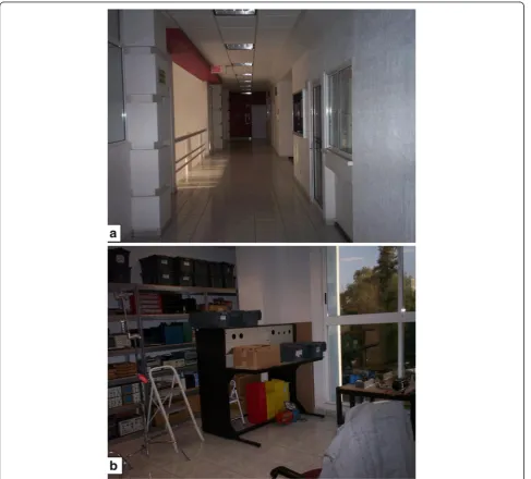
reflections. The radiating cable system was located inside a university building which has classrooms, laboratories, offices, and a warehouse. This building is a five-story structure where the interior and exterior walls were built
with drywall and block, respectively. Ceilings were built of steel decks and metallic beams, while the floors were built of ceramic tile. Ceilings are 4 m high with false ceilings of 3 m high. Figure 2 shows the corridor (a) and warehouse (b) of the measurement site.
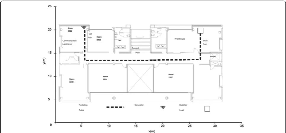
The radiating cable was placed over the false ceiling of the second level, and it was laid along three paths. The first path of the radiating cable was located over the communication laboratory. The second path was posi-tioned along the corridor, and the third path was placed over the warehouse. Figure 3 shows the layout of the second level indicating the placement of the radiating cable as well as the geographic reference used in this experiment. The communication laboratory has metallic shelves with typical equipment for radio communica-tions. Room 2204 contains tools and equipment to fabri-cate printed circuit boards. Rooms 2201, 2202, and 2207 contain school furniture such as benches, chairs, desks, and worktables. Finally, in the warehouse, there are many metallic objects, electronic components, and typ-ical equipment such as oscilloscopes, multimeters, and power supplies.
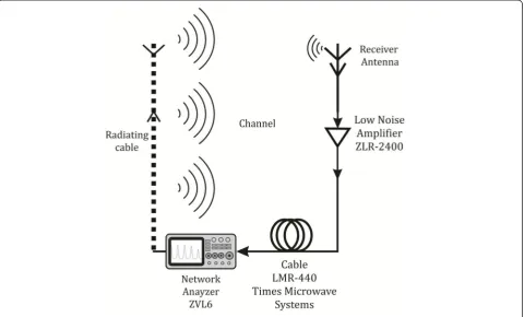
2.3 Measurements
The frequency response of the channel is obtained dir-ectly by the measurement system of Figure 4. The meas-urement system uses as a main device a vector network analyzer (VNA). The VNA is the ZVL6 model from Rohde and Schwarz (Munich, Germany). The radiating cable is plugged to port 1 of the VNA which applies a sweep of discrete frequenciesfk; wherefk=f0+kΔf, 0 <k<N, f0is the lowest frequency in the band of study,Δfis the
frequency sample spacing, and N is the number of
fre-quency samples. At the same time,Ncomplex samples of
the frequency responseH(k) are measured in the receiver antenna which is connected to port 2 of the VNA.
The measurements were achieved withf0= 1,300 MHz
and Δf= 0.5 MHz. The frequency response consists of
1,000 complex samples (N). Around 30 m of flexible low-loss coax cable (LMR-400 from Times Microwave Systems, Wallingford, CT, USA) were used to connect the receiver antenna with port 2 of the network analyzer. A low-noise amplifier (ZRL-2400 from Mini-Circuits, Brooklyn, NY, USA) was used between the wideband omnidirectional antenna of the receiver and the flexible low-loss coax cable. Additionally, the receiver antenna was placed 1.5 m high on a trolley which carried the power source for the low-noise amplifier.
The frequency response measurements were collected at fixed locations inside each room on the second floor of the building. In each room, around 120 frequency response samples were measured and recorded, and the separation between the frequency response samples was 10 cm. These samples were distributed throughout the test area. In the corridor case, samples were collected along three parallel paths to the second segment of the radiating cable. The surrounding environment was kept stationary during the measurements by avoiding the movement of objects and the presence of people.
2.4 Frequency-domain channel modeling
The measured frequency response can be understood as a random process; therefore, an AR model can map the frequency response samples into a limited number of
filter poles representing an AR process. An AR process of orderpis given by:
Hmeasðfn;xÞ−Xp
i¼1aiHmeasðfn−i;xÞ ¼V fð Þn ð7Þ
where Hmeas(fn,) is the nth sample of the measured
fre-quency response,V(fn) is a complex white noise process,
and the complex constants ai are the parameters of the
model. Taking the z-transform of Equation 7, the AR
process can be depicted as the output of a linear filter with a transfer function driven by a zero-mean white noise. The transfer function is given by:
G zð Þ ¼ 1
1þXp
i¼1aiz −1¼
Yp
i¼1 1
1−piz−1 ð8Þ
wherepiis theith pole of the transfer function.
The ai parameters are the solution for Yule-Walker
equations [11]:
Rð Þ−l −Xp
i¼1aiR ið Þ ¼−l 0; l>0 ð9Þ
in which R(k) is the frequency correlation function
de-fined in Equation6, andR(−l)= R(l). The variance of the
zero-mean white noise process V(fn) is the minimum
mean-square of the predictor output, which is given by:
σ2
v¼Rð Þ0 −
Xp
i¼1aiR ið Þ ð10Þ
In general, the order of the model depends on the measured site; however, the fifth-order process has been used as an upper bound [10].
Conventionally, a pole close to the unit circle denotes significant power at the frequency related to the angle of the pole. However, in the case of the AR frequency-domain model, a pole close to the unit circle means that there is significant power at the delay related to the pole angle. The delay is calculated as:
τ¼− θ
2πfs ð11Þ
where θis the angle of the pole, and fsis the frequency
step (0.5 MHz).
3 Results and analysis
Figure 5 depicts the obtained cumulative distribution of
rms delay spread for all measurements. It is observed
that the maximum value of the rms delay spread is
10 15 20 25 30 35 40 45 50
rms Delay Spread τrms
P
Figure 5CDF of thermsdelay spread obtained from wideband measurements and comparison with Gaussian and non-parametric distributions.
does not follow any particular distribution, and the
range of rms delay spread values is closely similar to
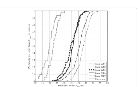
[7]. On the other hand, the cumulative distribution func-tions of the delay spread for every room have a smaller range of variations and different averaged values as shown in Figure 6.
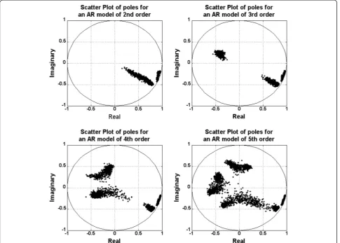
After various series of measurements, the corridor was found as the main site where the general characteristics of the channel can be determined (coherence bandwidth, delay spread, impulse response variation, etc.), since the poles in the corridor are a good approximation (in almost all magnitude and phase range) to the poles obtained in all rooms. Therefore, the results depicted in Figure 7 correspond to the scatter plots of the poles for models of orders 2, 3, 4, and 5 at the corridor. These results show that for all cases, there are two poles close to the unit circle with averaged angles of −0.3403 and −0.5394 rad which correspond to delays of 108.32 and 171.7 ns, respectively. According to the work reported in [10], two significant poles can be interpreted as two significant clusters of multipath arrivals. In this particular case, the
poles of the AR model of second order showed a defined behavior in the complex plane. This better-defined behavior showed the variation of the signal delay along the cable length. The magnitude of pole 1 was almost constant and its angle rotates clockwise, which represents the variation of the delay in receiver positions along the cable length. At the same time, pole 2 displayed a reduction of its magnitude and minimum variations of its angle. This describes the reduction of the τrms as the receiver moved away from the cable feeder in a direction parallel to the cable. Recall that in [10], the delay spread is
mainly related with the angles of both poles and less
closely with themagnitudeof the second pole.
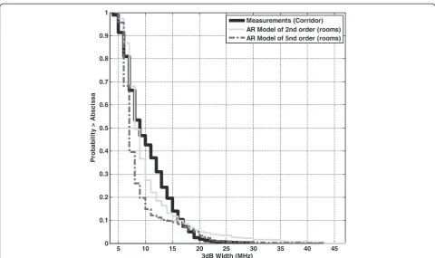
Figure 8 shows the complementary cumulative distri-bution functions of the 3-dB width of the correlation function for the measurements of corridor and room data generated with AR models of second and fifth orders. The statistics of the AR model of second order fits more closely to the experimental measurements and will be used to understand the relationship between the model poles and the behavior of the channel.
Figure 9 depicts the enlarged scatter plot of poles for the second-order model. Note that the poles show a shifting which corresponds to the position change of the receiver along the corridor. The arrow marks the direction of the shifting when the receiver is moved along the posi-tivex-axis fromx= 5 m tox= 25 m aty= 14 m (according to the layout of Figure 3). The clockwise shifting of pole 1 marks an increase of the delay of the first cluster of multi-path arrivals. Pole 2 has an almost null change in the angle, but a reduction of the magnitude is manifested. It implies a reduction of the span of the impulse response or the power delay profile along the corridor, and in
conse-quence, the rms delay spread is reduced. This situation
can be appreciated in Figure 10 from a point of view of the impulse response.
Figure 10 corresponds to the normalized impulse responses which were obtained along a parallel route to the radiating cable in the corridor. It illustrates how the impulse response starts with different delays. In the case
of x= 5 m and y= 14 m, the impulse response starts
around 15.5 ns; on the contrary, for x= 25 m andy= 14 m, the impulse response starts around 108 ns (refer to Figure 3 for both cases). Furthermore, the impulse re-sponses finish in a similar time. This fact explains the different mean values obtained from thermsdelay spread for every room (Figure 6). The former corresponds to the
area of the radiating cable which is near to the feeder and the latter corresponds to the opposite situation.
Note the strong dependence between the rms delay
spread and the length of the radiating cable as well as its best fit (Figure 11). This relationship along the corridor can be approximated as:
τrms≈50−3
2x ð12Þ
wherexis the position of the receiver along the corridor
given in meters, and τrmsis given in ns. An example of
this behavior can be seen in Figure 9, where the
magni-tude of pole 1 increases as the delay spread decreases. It was shown in [12] that without diversity or equalization, the ratio of thermsdelay spread to symbol duration in a digital transmission must be kept below 0.2 to have a tolerable intersymbol interference. Thus, assuming this criterion, in Room 2202, the maximum value ofτrmswas 54.4 ns, and therefore, the channel can support a data rate up to 3.6 Mb/s. Meanwhile in Room 2207, the maximum value ofτrmswas 28.5 ns; hence, the channel can handle a data rate up to 7 Mb/s. Such a situation must be considered in the design of modern wireless systems.
Finally, the relationship between the coherence band-widthBCandrmsdelay spreadτrmsthat was mentioned in
5 10 15 20 25 30 35 40 45 AR Model of 2nd order (rooms) AR Model of 5nd order (rooms)
5 10
15 20
25
0 100
200 300
400 0 0.5 1
Position x (m) [y=14 m]
Time (ns)
N
o
rm
a
liz
e
d
A
m
p
lit
u
d
e
t=15.5 ns t=108 ns
Δ
Δ
Figure 10Normalized impulse responses along the corridor.
0.2 0.3 0.4 0.5 0.6 0.7 0.8 0.9 1
-0.6 -0.5 -0.4 -0.3 -0.2 -0.1
Real
Im
ag
in
ar
y
Pole 1 Pole 2
receiver position x=5 m y=14 m
receiver position x=25 m y=14 m Shifting
of pole 1
receiver position x=5 m y=14 m Shifting
of pole 2 receiver
position x=25 m y=14 m
101.1 101.2 101.3 101.4 101.5 101.6 101.7 100
101 102
rms delay spread τrms (nsec)
C
o
rre
la
ti
o
n
3
d
B
W
id
th
(MH
z
)
Measurements Fitted Line
Figure 12Relationship betweenBcandτrms.
5 10 15 20 25
10 15 20 25 30 35 40 45 50 55
position x (m) y=14 m
rm
s del
ay sp
re
ad
τrm
s
(
n
s
)
rms delay spread (τrms) fitted line
Section 2 was found using a linear regression in logarithmic scale and is given by:
Bc≈ 1
τrms ð13Þ
Figure 12 shows the width (3 dB) of the frequency
correlation function versus its corresponding rms delay
spread and the best-fit line.
4 Conclusions
At the beginning of this paper, it was pointed out that radiating cables can be used as part of wireless systems such as in distribution systems, by providing coverage for in-building cellular scenarios, as well as in radio detection and wireless indoor-positioning systems. Nevertheless, modern digital communication systems require broad-band to be deployed. In this context, the study and design of any wireless system needs to know the multipath fading behavior of the channel in order to obtain an optimal performance of the system.
The coherence bandwidth and the rms delay spread
(τrms) were obtained by measuring the frequency response of the channel, and it was demonstrated that there is dependence between τrms and the receiver position along the cable length. This dependence must be taken into account in the design of broadband systems with mobility. Furthermore, such dependence can be used for wireless localization applications in indoor environments.
Moreover, an AR model for the frequency response was carried out. Complementary cumulative distribution functions showed that a second-order AR model gives the best fit at the 3-dB width of the frequency correlation function and showed a better-defined behavior in the complex plane. This better-defined behavior can be useful in the computer simulation of the channel or in the designing of simulation tools which allow evaluating specific systems under different schemas of modulation, coding, and equalization.
As it is known, the most modern wireless technologies are based on models because of the random variations of the wireless channel. Thus, the design and study of radiating cable systems can be carried out by using auto-regressive modeling of frequency response; however, it is necessary to implement more studies in different envi-ronments in order to compare and verify the channel behavior obtained in this study, including the effects of moving scatters.
Competing interests
The authors declare that they have no competing interests.
Acknowledgements
This work was partially supported by the Mexican Consejo Nacional de Ciencia y Tecnología (CONACYT), Project No. 154691. One of the authors, Jorge A. Seseña-Osorio wishes to thank the CONACYT for Scholarship Number 34612.
Author details 1
Instituto Nacional de Astrofísica Óptica y Electrónica (INAOE), Calle Luis Enrique Erro No. 1, Tonantzintla, Puebla C.P. 72840, Mexico.2Tecnológico de Monterrey, Campus Querétaro, Epigmenio González 500, Fracc. San Pablo, Santiago de Querétaro, Querétaro C. P. 76130, Mexico.3Tecnológico de Monterrey, Campus Monterrey, Av. Eugenio Garza Sada 2501 Sur, Col. Tecnológico, Monterrey, NL C.P. 64849, Mexico.
Received: 21 May 2014 Accepted: 6 January 2015
References
1. SEM Dudley, TJ Quinlan, SD Walker, Ultrabroadband wireless-optical transmission links using axial slot leaky feeders, and optical fiber for underground transport topologies. IEEE Trans. Veh. Technol.57(6), 3471–3476 (2008)
2. L Feng, X Yang, Z Wang, Y Li, The application of leaky coaxial cable in road vehicle communication system, inProceedings of 9th International Symposium on Antennas Propagation and EM Theory, 2010, pp. 1015–1018 3. I Stamopoulos, A Aragón-Zavala, SR Saunders, Performance comparison of
distributed antenna and radiating cable systems for cellular indoor environments in the DCS band, inProceedings of Twelfth International Conference on Antennas and Propagation, 2003, pp. 771–774
4. EUPEN AG Cable, URL: http://www.eupen.com/cable/rf/radiating/index.html. Accessed 12 May 2014
5. T Higashino, K Tsukamoto, D Komaki, Radio on leaky coaxial cable (RoLCX) system and its applications, inProceedings of PIERS, 2009, pp. 40–41 6. M Weber, U Birkel, R Collmann, J Engelbrecht, Comparison of various
methods for indoor RF fingerprinting using leaky feeder cable, in
Proceedings of 7th Workshop on Positioning Navigation and Communication (WPNC), 2010, pp. 291–298
7. YP Zhang, Indoor radiated-mode leaky feeder propagation at 2.0 GHz. IEEE Trans. Veh. Technol.50(2), 536–545 (2001)
8. Chehri, A., H. Mouftah, Radio channel characterization through leaky feeder for different frequency bands, in Proceedings of IEEE 21stInternational Symposium on Personal Indoor and Mobile Radio Communications, Istanbul, Turkey, 26–30 Sept 2010. pp. 347–351.
9. G Gu, X Gao, J He, M Naraghi-Pour, Parametric modeling of wideband and ultrawideband channels in frequency domain. IEEE Trans. Veh. Technol. 56(4), 1600–1612 (2007)
10. SJ Howard, K Pahlavan, Autoregressive modeling of wide-band indoor radio propagation. IEEE Trans. Commun.40(9), 1540–1552 (1992)
11. K Pahlavan, AH Levesque,Wireless Information Networks, 2nd edn. (Wiley & Sons, Chichester, West Sussex, UK, 2005)
12. JCI Chuang, The effects of time delay spread on portable radio communications channels with digital modulation. IEEE J. Sel. Areas Commun.5(5), 879–899 (1987)
Submit your manuscript to a
journal and benefi t from:
7Convenient online submission
7Rigorous peer review
7Immediate publication on acceptance
7Open access: articles freely available online
7High visibility within the fi eld
7Retaining the copyright to your article