R E S E A R C H
Open Access
A computationally efficient method for
self-planning uplink power control parameters
in LTE
José Ángel Fernández-Segovia
1*, Salvador Luna-Ramírez
1, Matías Toril
1, Ana Belén Vallejo-Mora
1and Carlos Úbeda
2Abstract
Uplink power control has a strong impact on the performance of mobile communication networks. In this work, an automatic parameter planning algorithm for the standardized power control scheme in the physical uplink shared channel (PUSCH) of long term evolution LTE is proposed. The method is conceived for the network design stage, when network measurements are still not available. The proposed heuristic algorithm can handle irregular scenarios at a low computational complexity. For this purpose, the parameter planning problem in a cell is formulated
analytically through the combination of multiple regular scenarios built on a per-adjacency basis. Method assessment is carried out over a static system-level simulator implementing a real scenario. Results show that the proposed method can improve average user throughput and cell-edge user throughput when compared to current vendor approaches, which provide network-wide uniform parameter settings.
Keywords: Mobile network; Self-planning; LTE; Uplink power control; Real network sensitivity analysis
1 Introduction
Network planning plays a very important role in cellular communication networks. Before deployment, a thorough analysis must be done to achieve an adequate trade-off between capacity and coverage in the service area and pre-dict future problems. A proper network planning avoids problems during the operational stage, minimizing (or, at least, delaying) subsequent capital investment [1,2].
Regardless of the radio access technology, cellular net-work planning is divided into core netnet-work planning and radio access network (RAN) planning. While the former is often only a dimensioning process, the latter entails the definition of RAN parameter settings that can be deployed in the roll-out stage. These parameters include not only physical parameters (e.g., site positions, antenna bearings, or power amplifier limits) but also logical parameters in radio resource management (RRM) algorithms [3-5]. In the past, due to the complexity of finding optimal set-tings for each specific scenario, vendors have provided
*Correspondence: [email protected]
1Ingeniería de Comunicaciones, Universidad de Málaga, Campus de Teatinos S/N, 29071 Malaga, Spain
Full list of author information is available at the end of the article
operators with safe recommended values that should work reasonably well in most cases. Thus, the flexibility given by network parameters has not been fully exploited. To solve this situation, an effort has been made in the 3rd Gen-eration Partnership Project (3GPP) long term evolution (LTE) standard to define the requirements for automating and improving network planning [6]. Likewise, automatic (or self-) planning has been identified by the industry as a key process in self-organizing networks (SON) [7-9].
Uplink power control (ULPC) is an important RRM process in mobile networks, as it has a direct impact on received signal and interference levels, as well as on user battery consumption. This makes ULPC an ideal candi-date for automated parameter planning. In practice, the variability of propagation, traffic and interference condi-tions make it very difficult for operators to find optimal settings for these parameters before operation. For this reason, operators usually set ULPC parameters to safe values, which are deployed network wide. As a result, sub-optimal network performance is obtained due to network irregularities. Even if this can be solved later during net-work operation, the provision of proper initial settings is greatly appreciated by operators.
In the literature, several power control schemes have been proposed. Fractional power control (FPC) has been selected for the physical uplink shared channel (PUSCH) in LTE [10,11]. A performance analysis of open-loop FPC is presented in [12,13]. Such an analysis is extended in [14-16] to closed-loop behavior. Later studies have evalu-ated more sophisticevalu-ated power control schemes for LTE, which take into account interference and load condi-tions [17,18]. In [19], a parameter sensitivity analysis for the standardized FPC algorithm is carried out based on system-level simulations. As a result, a suboptimal parameter configuration is suggested for interference-limited and noise-interference-limited macro-cellular scenarios. How-ever, finding the best parameter configuration for every cell in the network is a more challenging task, since the underlying problem is a large-scale separable non-linear optimization problem. In [20], the adjustment of ULPC parameters in a single cell is formulated as a clas-sical optimization problem with average throughput and cell throughput as alternative figures of merit. The latter analysis is extended to a multi-cell scenario in [21] by for-mulating ULPC as a non-cooperative game model. Then, a heuristic iterative optimization algorithm is proposed, where cells report UL power settings to the network management system and exchange power and interfer-ence information with their neighbor cells. In [22], a self-planning method is proposed for selecting the best parameter settings in FPC on a per-cell basis in an irregu-lar LTE scenario. The proposal is based on an exhaustive search approach using Taguchi’s method over a system-level simulator. A more computationally efficient planning method is presented in [23]. The core of the method is an analytical model that predicts the influence of the nominal power (a.k.a. power offset) and path-loss compensation factor on call acceptance probability for a given spatial user distribution. A suboptimal value of these parame-ters is computed on a per-cell basis by a randomized local greedy search algorithm. Alternatively, other studies con-sider tuning algorithms for the network operational stage. For instance, a self-tuning algorithm is proposed in [24] to dynamically adjust nominal power parameter based on overload indicator [25] so as to control the overall interfer-ence in the network. Similarly, in [26], a self-tuning algo-rithm for FPC is proposed based on fuzzy-reinforcement learning techniques. These self-tuning algorithms, con-ceived to be executed during network operation, can also be applied to network planning, provided that a system performance model is available. However, most self-tuning algorithms rely on iterations that require eval-uating system performance for many different parameter settings. This iterative process is straight-forward for live networks due to the availability of performance measure-ments. However, this is not the case of network planning, where computations required to measure the quality of
a new parameter plan at every iteration may jeopardize method scalability when large scenarios are considered. For this reason, most ULPC planning methods in the literature rely on simple analytical models for system per-formance assessment. To the authors’ knowledge, few of them can handle irregular scenarios at a low com-putational cost and none of them considers closed-loop performance.
In this paper, a self-planning algorithm for ULPC parameters in the PUSCH of LTE is proposed. The self-planning algorithm determines the maximum uplink cell load,UUL, and the nominal PUSCH power parameter in FPC,P0. Full path-loss compensation is assumed in this work (i.e., FPC parameterαis fixed to 1), as implemented in most first vendor releases. To deal with network irreg-ularities, the parameter tuning problem is solved on a cell-by-cell basis by aggregating the results from multi-ple regularized scenarios built on a per-adjacency basis. Such a regularization approach reduces the size of the solution space, thus reducing the time complexity of the method. Both open-loop and closed-loop power con-trol performance are considered in the problem model. Method assessment is carried out over a static system-level simulator implementing a real network scenario. The main contributions of this work are as follows: a) a thorough parameter sensitivity analysis of ULPC closed-loop performance in a realistic simulated scenario and b) a self-planning method for ULPC parameters that can handle irregular scenarios at a low computational com-plexity and considers both open- and closed-loop ULPC performance. Similar to [23], the proposed heuristic algo-rithm can handle irregular scenarios while still using a semi-analytical approach. Unlike [23], the optimized parameters are the nominal power and the maximum cell load, instead of the path-loss compensation factor. More importantly, the method proposed here has bet-ter scalability and computationally efficiency due to the regularization approach. The rest of the paper is orga-nized as follows. Section 2 outlines the LTE system model used in the planning process. Section 3 describes the design of the proposed planning algorithm. Section 4 presents simulation results obtained in a real network scenario. Finally, Section 5 presents the concluding remarks.
2 Uplink system model
algorithm and the physical resource block (PRB) alloca-tion scheme, are modeled in this work.
2.1 Power control algorithm
The aim of power control is to adjust the transmit power of the user equipment (UE) to fulfill quality of service (QoS) requirements at the base station (i.e., eNodeB, eNB). The power control scheme for PUSCH combines an open-loop and a closed-loop algorithm. The former aims to compensate for slow channel variations, while the latter adapts to changes in the inter-cell interference conditions, or measurement and power amplifier errors. In the stan-dardized algorithm [11], the UE transmit power (in dBm) is given by
where Ptxmax is the maximum UE transmit power, α is
the channel path-loss compensation factor (set to 1 in this work),PLare the propagation losses,MPUSCH is the number of PRBs assigned to the UE, andTF +f(TPC)
is a dynamic term that depends on the selected modu-lation scheme and power-control commands sent by the eNB. Equation 1 consists of three parts: a basic open-loop operating point, a dynamic offset controlled by closed-loop operation, and a bandwidth correction factor. The open-loop term consists of a semi-static level given by the parameterP0(known as nominal power), defining the average received signal level target for all UEs in a cell, and a path-loss compensation term, controlled by path-loss compensation factor,α. From (1), it follows that setting
P0controls UE transmit power, thus determining the per-ceived signal-to-interference-plus-noise ratio (SINR) in the serving cell and the interference level in surrounding cells.
2.2 PRB allocation scheme
The PRB allocation scheme also has a strong impact on UL performance. PRB allocation is done by a scheduler in the eNB, which assigns PRBs to users so as to maxi-mize average cell throughput while keeping cell-edge user throughput within reasonable limits. For mathematical tractability, a simplified scheduling algorithm consisting of two stages is used in this work. It is assumed that a) full spectral sharing is used (i.e., frequency reuse is 1), b) radio resources are independently allocated between cells (i.e., PRB allocation is done on a cell basis), c) users are uniformly distributed in a cell, but unevenly dis-tributed among cells, and d) any user has infinite data to
transmit (i.e., full buffer service model). In a first stage, referred to as naivescheme, a preliminary PRB assign-ment is made based on the open-loop power control algorithm. Thus, an estimate of the maximum number of PRBs assigned for each user is obtained, from which PRB usage and average interference levels can be pre-dicted. Then, a second scheme, referred to as refined
scheme, considers the closed-loop power control algo-rithm. With the latter scheme, the final PRB assignment guaranteeing a minimum SINR is computed based on interference estimates with the PRB assignment suggested by the first naive scheme. Both schemes are described next.
2.2.1 Naive scheme - interference estimation
A theoretical PRB allocation scheme is first computed based on open-loop power control. A grid of positions in a cell is defined, so that each position represents a poten-tial user. The number of PRBs assigned to userk,M(k), is the maximum number of PRBs that can be assigned to the UE located at that point while still guaranteeingP0at the serving eNB, computed as
whereMminandMmax are the minimum and maximum number of PRBs that can be assigned to the UE, defined as network wide settings, PL(k) are propagation losses (including antenna gains and path loss) for user k, and
P0(S(k))is the value ofP0for the cell serving userk,S(k). In this work, Mmin=2 and Mmax ranges from 6 to 100 depending on system bandwidth [28]. The value ofM(k)
obtained by (2) is used to compute the transmit power for each user,PTX(k), as in (1). Then, the UL interference level received at each eNBi,IUL(i), is calculated as the sum of the interference from every neighbor cellj and thermal noise. The interference from each neighborjis calculated as the average received signal level from UEs in that neigh-bor, weighted by the uplink cell load, UUL(j). UUL(j) is given by the PRB utilization ratio (i.e., the number of used PRBs divided by the number of available PRBs for a period of time). Thus, the number of users (locations) in the service area ofj, and
2.2.2 Refined scheme - SINR estimation
Based on estimated interference levels, a second and more accurate PRB allocation defines the maximum number of PRBs while still satisfying a minimum SINR threshold, computed as
and SINRth is the minimum SINR value to be satisfied (−2.8 dB in this work [28]). Equation 4 shows how the number of PRBs assigned to a user changes with radio link conditions (i.e.,PLandIUL). A user experiencing good radio conditions (i.e., low path-loss and low interference level) can be assigned all available PRBs,Mmax. However, as path-loss and/or interference increases, the number of PRBs allocated to the user is reduced in (4). This PRB reduction allows a higher transmission power per PRB, and thus, the minimumSINRthreshold is fulfilled.
2.3 Key performance indicators (KPI)
Several indicators are calculated to check user and net-work performance with different ULPC parameter set-tings. The maximum throughput per PRB achieved by a user is obtained from SINR values by the truncated Shannon bound formula [29] as
THperPRB(k)= THperPRBmax SINRmax<SINR(k),
(5)
whereTHperPRBmaxis the maximum throughput per PRB achievable by the codeset,SINRmaxandSINRminare SINR values where maximum and minimum throughputs are reached, andβis a constant. Then, the maximum achiev-able throughput is computed by multiplying throughput per PRB by the number of assigned PRBs obtained in (4). In this work,THperPRBmax= 514 kbps,SINRmax= 14 dB, SINRmin=−9 dB andβ=0.6.
Average user throughput, THavg, is used as a mea-sure of cell capacity, while cell-edge user throughput,
THce, is used as a measure of cell coverage. Average user throughput is obtained as the average of individual user throughputs in the serving area of a cell, as
THavg(i)=
∀k∈A(i)M(k)·THperPRB(k)
Nu(i) ·UUL(i).
(6)
A user location,k, is assigned to celliif the latter is the one providing the minimum propagation losses. Cell-edge user throughput,THce(i), is defined as the fifth percentile of user throughput in the cell (i.e., the user throughput value exceeded by 95% of user locations in celli).
3 Self-planning method
In this section, an algorithm for the automatic planning of the nominal power,P0, and maximum UL cell load,UUL, on a cell basis is presented. Firstly, a qualitative analysis of the influence of these parameters on network coverage and capacity is presented. Then, a preliminary parame-ter sensitivity analysis is performed in a regular scenario. From this quantitative analysis, the basic principles of the optimization algorithm are derived. The extension of the algorithm to deal with irregular scenarios is detailed later. With such an extension, ULPC settings can be adjusted on a per-cell basis to achieve better network performance.
3.1 General considerations
In mobile communication systems, coverage and capac-ity cannot be optimized independently as one affects the other. Network performance is a trade-off between cell-edge users, defining system coverage, and cell-center users, which have a larger influence on system capacity. This trade-off is the subject of the coverage-capacity opti-mization (CCO) problem, which has been identified as a relevant SON use case by 3GPP [30].
CCO can be performed by tuning ULPC parameters. Setting the average received signal level at the eNB,P0, has a direct impact on the performance of both the adjusted cell and its surrounding cells. In the considered cell, a large value of P0 enforces high transmit power for all users. Thus, users closer to the eNB should experience higher SINR values and, consequently, better UL performance. This is translated into higher peak user throughput in the cell at the expense of more user battery consumption. In contrast, cell-edge users that are power-limited cannot increase their transmit power when increasingP0. At the same time, cell-edge users in surrounding cells experience low SINR due to increased interference level. Conversely, a lowP0value favors cell-edge users in surrounding cells at the expense of cell-center users in the adjusted cell. Alternatively, UL cell load, UUL, can be limited in a cell to avoid interference problems in surrounding cells. Con-trol of UUL can be implemented by traffic management procedures, such as call admission control or cell load sharing.
The optimal P0 andUUL settings in a cell are highly influenced by the propagation scenario and traffic dis-tribution in both the cell under study and its neighbors. Therefore, any CCO algorithm must consider scenario irregularities and deal with neighbor cell conditions. As a consequence, CCO becomes a large scale non-separable multivariate optimization problem, where all cells must be jointly optimized. The size of the solution space is (NvP0 ·NvUUL)Nc, where NvP0 andNvUUL are the number
which are substituted by heuristic algorithms. To reduce the search space, some approaches only evaluate a limited set of representative parameter combinations, selected by, e.g., Taguchi’s method [22]. Other approaches build an initial solution by assuming that all cells have the same parameter settings, which is then refined by a randomized local search process, e.g., greedy search [23] or simulated annealing. Even the latter approach requires many itera-tions to obtain soluitera-tions of reasonable quality, since any parameter change in a cell affects the performance of sur-rounding cells, and each iteration requires evaluating the overall network performance in the whole scenario after every parameter change.
In this work, a different approach is followed to reduce the search space. The global multi-variate optimization problem is divided intoNcindependent bi-variate opti-mization sub-problems (one per cell), each providing a sub-optimal solution for a cell i, P0(i) and UUL(i). To decouple sub-problems, some approximation is taken to model the irregular local scenario in the cell under study by a regular one. The idea is to approximate one real and complex scenario by many simple and regular scenarios that can be solved easily and independently. Apart from reducing the solution space, regularizing the scenario has other important advantages from the computational per-spective: a) the grid resolution needed to obtain accurate propagation predictions is lower for regular scenarios than for irregular ones, and b) interference calculations for neighbor cells can be replicated due to the symmetry in a regular scenario, whereas these have to be treated individ-ually in an irregular scenario due to the lack of symmetry. The following subsections describe first the optimiza-tion process in a regular scenario and later explain the extension to irregular scenarios.
3.2 Regular scenario
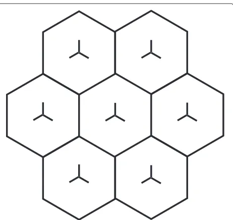
A preliminary sensitivity analysis shows the impact of tuning P0 and UUL on network performance in a reg-ular scenario. For this purpose, a static system-level simulator is used. The simulation scenario, shown in Figure 1, consists of one central tri-sectorized site sur-rounded by a first tier of tri-sectorized neighbor sites. Main simulation parameters are shown in Table 1. Per-formance statistics are collected only for the central celli.
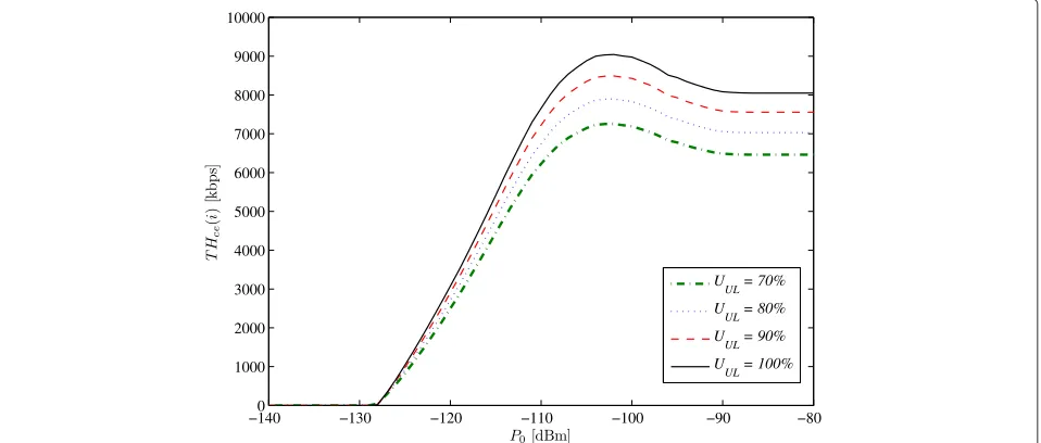
Network performance is evaluated for uniformP0and UULsettings in the scenario (i.e., all cells share the same parameter values). Figure 2 and Figure 3 show cell-edge and cell-average user throughput for celli, THce(i) and
THavg(i), with different P0 and UUL settings. Increas-ingP0leads to higher PTX(k) for cell-center users, thus increasing average user throughput. This improvement is limited by the interference from users in other cells, also increasing theirPTX(k)in this regular scenario. Thus,
Figure 1Regular scenario in the parameter sensitivity analysis.
THavg(i)reaches a maximum value, after whichTHavg(i) decreases. The largest value of THavg(i) is obtained for high values ofP0(i.e.,−102 dBm), where cell-center users can make the most of low propagation losses and received interference level is not much larger than the noise floor. In contrast, cell-edge performance quickly degrades asP0 increases. This is due to the fact that cell-edge users reach their power limit, so that their transmit power does not change, but interference increases, as users in other cells increase their transmit power in the regular scenario. As a consequence, the maximum value forTHce(i)is reached for low values ofP0, whenIUL(i)is close to the noise floor
Table 1 Simulation parameters
Parameters Settings
Spectrum allocation 10 MHz (50 PRBs)
Carrier frequency 2 GHz
Cell layout 7 eNBs, 21 sectors, regular grid
(200 m resolution). Distance attenuation 133.9+35.2log10(d),din km
Slow fading constant 8 dB
Thermal noise density −174 dBm/Hz
Cell radius 1.5 km (3 km inter-site distance)
eNB antenna height 30 m
eNB antenna tilt 5◦
eNB antenna pattern and gain 3GPP ideal [32]
Maximum UE transmit power 23 dBm
Path-loss compensation factor,α 1 (full compensation)
Figure 2Cell-edge throughput performance in regular scenarios with uniformP0andUUL.
(i.e.,−119.4 dBm). Note that smallP0deviations from the optimal value cause large deviations inTHce(i), but near-optimal performance inTHavg(i). This is evidence that the trade-off between coverage and capacity is more critical for cell-edge users.
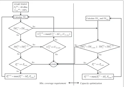
Based on the behavior observed in Figure 2 and Figure 3, a self-planning algorithm forP0andUULin a regular sce-nario is designed. The flow diagram of the proposed iter-ative algorithm is shown in Figure 4.P0(n)andUUL(n)denote parameter values in iterationn. The optimization engine is a simple gradient-based local optimization method, whose aim is to maximize the average user throughput,
THavg(i), while keeping cell-edge throughput over a mini-mum,THce(i) >THce,min. Such a formulation of the CCO problem can be found in the literature (e.g., [31]). For this
purpose,P0andUULare initially configured to arbitrar-ily high values (e.g., −80 dBm and 100%, respectively). Then, the algorithm iteratively decreases parameter val-ues. In a first stage, when minimum cell-edge throughput is not fulfilled (i.e., THce(i) < THce,min) and maximum THce(i) value has not been reached, the optimization engine tries to increase THce(i) by decreasing P0. Once coverage constraints are fulfilled (i.e.,THce(i)≥THce,min), the optimization engine keeps decreasingP0with the aim of maximizing THavg, until THavg(i) starts to decrease (i.e., optimalP0in terms ofTHavg(i)has been surpassed) or cell-edge throughput has become less than the mini-mum threshold. UUL is only decreased when minimum cell-edge throughput is not fulfilled. This is the case of interference-limited scenarios, consisting of very small
Figure 4Flow diagram of optimization process.
cells. ReducingUULonly when strictly needed is in line with operator policies, which only consider limiting the average PRB utilization in a cell under critical interference situations.
3.3 Irregular scenario
The above-described optimization algorithm is designed for a regular scenario, resulting in a solution where all cells have the same value ofP0andUUL. However, in live net-works, propagation, traffic, and interference conditions greatly vary among cells. These irregularities translate into uneven parameter configuration for optimal network per-formance. The following paragraphs describe a method to deal with such irregularities. The method consists of four stages, namely global scenario construction, division into local regular scenarios, local problem solving, and aggregation of local solutions.
3.3.1 Global scenario construction - adjacency definition The method starts by collecting network configuration data, consisting of site locations, antenna height, and antenna bearings (i.e., azimuth and tilt). This data is included in propagation models to define a list of relevant
non co-sited neighbor cells for every cell in the sce-nario. Such a list is used later for regularization of local scenarios, as will be explained later.
Several options could be used to automatically define neighbors for every cell in the scenario. Relevant neigh-bors are usually identified by computing the con-tribution that every single user in each candidate neighbor cell has on the UL interference of the cell under study. In the absence of real measurements, this calculation requires computing a point-by-point path loss matrix, from which to identify cell dominance areas, which increases the computational load of the method.
For computational efficiency, a simple automatic neigh-bor definition algorithm is used here with planning pur-poses. The aim is to rank non co-sited neighbors by relevance assuming that the average path loss of all users in a neighbor cell is similar to that from neighbor eNB location. The number of neighbors must be kept within reasonable limits. An intuitive indicator for neighbor relevance in the UL,NRUL, is defined as
whereL(i,j)is the path loss between the cell under study
i and cell j computed by some propagation model, and
Ah(i,j) and Av(i,j) are the horizontal and vertical gains for the antenna of cellito the location of eNBj. Roughly, the closest eNBsjin terms of electrical distance tend to give the lowestNRUL(i,j)values and are labeled as rele-vant neighbors of celli(i.e.,j∈Nr(i), whereNr(i)is the list of relevant non co-sited neighbors of celli). To limit the number of relevant neighbors, neighborsjhavingNRUL10 dB larger than that of the most relevant neighbor are dis-carded. For the same reason, a maximum of 12 neighbors per cell is configured.
3.3.2 Division into local regular scenarios
Once neighbors have been defined for each cell, the opti-mization process can start. Global network optiopti-mization is broken down intoNclocal optimization sub-problems, which are solved independently. Every sub-problem is solved by the regularization of one or several local scenar-ios. Two alternatives are considered, depending on how the regular local scenario is built for a celli:
• Mean radius approximation (MRA): A regular sce-nario, as that in Figure 1, is built for the cell under study i. Inter-site distance (ISD) in the regular sce-nario is taken from the global scesce-nario by averaging ISDs between the site of celliand the site of its neigh-bors in the real irregular scenario, excluding co-sited cells. Thus, MRA assumes a single ‘average’ regular scenario per cell. Then, optimalP0(i)andUUL(i)
val-ues for celliare obtained by applying the optimization method described in Figure 4 to this equivalent regular scenario.
• Adjacency-based approximation (AA): The optimiza-tion problem for celliis broken down intoNneigh(i)
sub-problems, where Nneigh(i) is the number of non
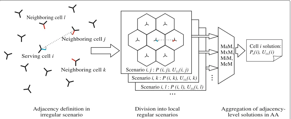
co-sited neighbors of celli (i.e., the length ofNr(i)). For each pair of cells(i,j), where i is the optimized cell andjis the selected neighbor, a regular scenario is built, as shown in Figure 5. ISD in the scenario is the one between cellsiandjin the real network. In the figure, it is observed how the relative position (i.e., dis-tance and antenna bearing angles) of cells in the real network is maintained. As a result of problem division,
Nneigh(i)regular scenarios are built and solved for each celli.
Note that MRA needs a single optimization process per cell, whereas AA requiresNneigh(i)optimization pro-cesses (one per neighbor). As a result, Nneigh(i) pairs of sub-optimal P0 and UUL values are obtained for each cell i, (P0(i,j), UUL(i,j)). Some aggregation pro-cess is then needed to obtain a single solution per cell, (P0(i),UUL(i)).
3.3.3 Aggregation of adjacency-level solutions in AA A single value of (P0(i), UUL(i)) is computed from all sub-optimal solutions involving cell i, where cell i is either source or target in the adjacency, i.e., (P0(i,j), UUL(i,j)) and (P0(l,i),UUL(l,i)). Four alternative aggrega-tion criteria are defined, namely maximum, mean, min-imum, and mixed. In each criterion, the final solution per cell is computed from adjacency-level solutions as follows: • Mixed method (MxM). This approach uses the maxi-mum criterion forP0(i), defined in (8), and the
mini-mum criterion forUUL, defined in (13). The aim is to
maximize SINR by selecting a largeP0 value, even if
interference is thus increased. Then, the lowestUULis
selected to mitigate such an interference increase.
Figure 6 summarizes the whole optimization process for a cell i in the AA method, including regularization on a per-adjacency basis, sub-problem solving and solution aggregation.
3.4 Computational complexity
a)
b)
Figure 5Scenario regularization.(a)Irregular scenario and(b)regularized scenario.
The time complexity of the AA self-planning algorithm is also O(Nc), since the number of sub-problems grows linear with the total number of relevant non co-sited neighbors in the scenario, which is proportional to the number of cells in the network.
4 Performance analysis
The solutions of the different variants of the proposed algorithm are tested in a system-level simulator imple-menting a real irregular scenario. The simulator includes all UL functionalities described in Section 2. For clar-ity, the analysis set-up is described first and results are presented later.
4.1 Analysis setup
The considered scenario consists of 233 sites (699 cells) in a large metropolitan area. Location, azimuth, and antenna
tilts are obtained from live network configuration data. ISDs range from 0.3 to 6 km. Other simulation parameters are shown in Table 1.
Five different self-planning approaches are tested. A first method uses MRA with neighbor cell selection as described in Section 3.3.1 (referred to as MRA). The other four methods use AA for dealing scenario irreg-ularities, considering MaM, MeM, MiM, and MxM as solution aggregation criterion, respectively. To quantify the benefit of tuning ULPC parameters on a cell-by-cell basis, uniform settings (i.e.,P0(i) = P0(j)andUUL(i) = UUL(j),∀i,j) are also tested. In this case, a set of bench-marking solutions is constructed by selecting different combinations ofP0andUUL.
To assess the value of a parameter plan, two per-formance indicators are used: a) as a measure of net-work capacity, overall average user throughput,THavg(i),
Scenarioi, l P (i, l), U (i, l): UL
Serving celli
Neighboring cellj
Scenarioi, j P (i, j), U (i, j): UL
Neighboring cellk
Neighboring celll
MaM, MxM, MiM, MeM
Cell solution:i P (i), U (i)0 UL
Scenarioi, k P (i, k), U (i, k): UL
...
...
Adjacency definition in irregular scenario
Division into local regular scenarios
Aggregation of adjacency-level solutions in AA
computed by averaging THavg(i) across cells in the sce-nario, and b) as a measure of coverage, the ratio of cells fulfillingTHce(i) > THce,min, denoted asRTHce,min. In this
work, THce,min = 100 kbps, based on typical operator demand.
4.2 Results
The analysis is first focused on network performance obtained with uniform parameter settings. Then, the anal-ysis proceeds to cell-based solutions obtained by the pro-posed self-planning methods. Finally, execution time is analyzed.
4.2.1 Uniform parameter settings
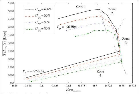
Figure 7 shows the coverage-capacity trade-off achieved with uniform P0 and UUL settings. Each point in the figure corresponds to a network parameter plan. Differ-ent curves correspond to differDiffer-entUULvalues (i.e., 70%, 80%, 90%, and 100%) and points in the curve correspond to P0 values ranging from−125 dBm (down and left in the figure) to−90 dBm (up and left). Note that network performance is better in the upper right area of the figure. Four regions are defined in every curve, corresponding to different network behaviors, denoted as zone 1 (P0 ≥ −
105 dBm), zone 2 (P0∈(−105,−115] dBm), zone 3 (P0∈ (−115,−119] dBm), and zone 4 (P0<−119 dBm).
WhenP0is extremely high (zone 1), both coverage and capacity indicators improve asP0decreases. In this situa-tion, interference levels are well above the noise floor, so decreasingP0in a cell and its neighbors decreases inter-ference by the same amount. As a consequence, cell-edge throughput improves, while throughput for cell-center users is maintained as both interference and desired signal level decreases. When P0 is medium (zone 2), a trade-off between coverage and capacity exists. Cell-edge throughput improves as P0 further decreases at the expense of degrading network average throughput. Lower values ofP0(zone 3) cause interference levels fall below the noise level, so that there is no benefit on fur-ther decreasing interference. On the contrary, cell-edge throughput starts to degrade. Finally, a strong degrada-tion in network performance occurs when P0 becomes less than the noise floor, −119.4 dBm in this work (zone 4).
The influence ofUULcan be seen by comparing curves in Figure 7. It is observed that curves are shifted up and left whenUULincreases. When more UL radio resources are available, users can reach higher throughput (i.e.,
THavg(i)increases), but interference levels also increase, and henceRTHce,min decreases.
4.2.2 Non-uniform parameter settings
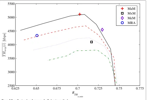
Figure 8 compares the performance of the different self-planning proposals for cell-based ULPC parameter settings. For comparison purposes, results of uniform parameter plans are superimposed. Axis scales have been adjusted for optimal viewing in the figure. Note that MiM is not shown, since MiM experiences a very poor network performance (i.e.,THavg(i)= 1,254 kbps andRTHce,min =
205/699 = 0.29). This is due to the fact that MiM sets
P0(i)to very low values, thus degrading SINR even for the best users. Other solutions (i.e., MaM, MeM, MxM, and MRA) perform similar to the best network performance with uniform settings (i.e., top-right in the figure). The best average throughput performance is achieved by MaM (i.e.,THavg(i)= 5,113 kbps), which outperforms MeM and MRA by 11.15% and 15.27%, respectively. MaM selects the maximum value ofP0 andUULacross adjacencies, thus achieving better overall throughput. As a drawback, inter-ference problems are greater, as pointed out by the lower value ofRTHce,min compared to other methods. The best
cell-edge throughput performance is achieved by MeM
(i.e.,RTHce,min= 0.73), which outperforms MaM and MxM
by 3.87% and 2.04%, respectively. Although MxM was designed as an intermediate solution between MaM and MiM, it is observed that limitingUULin MxM has a strong impact on average user throughput, which is 19.89% and 11.09% lower than those achieved by MaM and MeM, respectively. MeM outperforms all other methods, as it is the only solution achieving a coverage-capacity trade-off better than that obtained with any regular parameter setting.
4.2.3 Execution time
All methods were executed in an Intel® Xeon© computer with 3.47-GHz clock frequency and 12 GB of RAM. The time required to build the curve for uniformP0andUUL settings in the static system-level simulator was 2,500 s. In contrast, any of the self-planning methods proposed for constructing cell-based parameter plans took only 300 s in average (i.e., 0.43 s per cell).
It is also worth mentioning that, if a multi-variate exhaustive search approach is used, the addition of a new cell to an existing (i.e., already planned) scenario needs complete re-simulation of the whole scenario to build the new curve for uniform parameter settings. In
contrast, the self-planning method proposed in this work only needs solving 1+Nneigh(i)sub-problems (i.e., the re-computation of the new cell and its relevant neighbors) with regular scenarios.
5 Conclusions
In this work, a novel self-planning algorithm for UL power control parameters in the PUSCH of LTE has been presented. In the algorithm, the global network parameter optimization problem is divided into multiple simple optimization problems, one per adjacency, where a regular scenario is assumed. In such regular scenar-ios, a simple gradient descent method is used to find the optimal parameter settings that maximize average user throughput while still ensuring a minimum cell-edge user throughput. Then, the best parameter settings for each cell are calculated by aggregating adjacency-level solutions. Thus, the proposed heuristic algorithm can deal with irregular scenarios at a low computational complexity, which is critical for planning large scenar-ios. Performance assessment has been carried out over a static system-level simulator implementing a real sce-nario. Results show that averaging solutions across adja-cencies (i.e., MeM aggregation method) achieves the best trade-off between coverage and capacity, outperforming uniform network configurations for nominal power and UL cell load parameters.
The proposed self-planning algorithm can be imple-mented as part of a centralized SON system, which com-municates with the network management system (NMS). For an initial operational network stage, self-configuration can be performed by automatically retrieving ULPC parameters from the NMS. Later, every time a new eNB is added, the network self-planning algorithm can be re-launched. For this purpose, the new eNB sends its location and antenna configuration parameters to the NMS, which updates network topology in the SON server. Then, the SON server computes the new ULPC parameter configu-ration, which is sent to NMS so that it can be retrieved by the new eNB.
Competing interests
The authors declare that they have no competing interests.
Acknowledgements
This work has been funded by the Spanish Ministry of Economy and Competitiveness (TIN2012-36455), Optimi-Ericsson and Agencia IDEA (Consejería de Ciencia, Innovación y Empresa, Junta de Andalucía, ref. 59288) and FEDER.
Author details
1Ingeniería de Comunicaciones, Universidad de Málaga, Campus de Teatinos
S/N, 29071 Malaga, Spain.2Ericsson, Via de los Poblados 13, 28033 Madrid,
Spain.
Received: 28 October 2014 Accepted: 4 March 2015
References
1. A Hoikkanen, inInternational Conference on Wireless and Optical Communications Networks, WOCN. Economics of 3G Long-Term Evolution: the business case for the mobile operator (Singapore, July 2007), pp. 1–5 2. F Gordejuela-Sanchez, J Zhang, inIEEE Global Telecommunications
Conference, GLOBECOM. LTE Access network planning and optimization: A service-oriented and technology-specific perspective (Hilton Hawaiian Village, Honolulu, Hawaii, USA, December 2009), pp. 1–5
3. J Lempiainen, M Manninen,Radio Interface System Planning for GSM/GPRS/UMTS. (Springer, New York, NY, USA, 2001)
4. J Laiho, A Wacker, T Novosad,Radio Network Planning and Optimisation for UMTS. (John Wiley & Sons, New York, NY, USA, 2002)
5. AR Mishra,Advanced Cellular Network Planning and Optimisation. (John Wiley & Sons, New York, NY, USA, 2006)
6. 3GPP TS 32.500, Telecommunication management; Self-Organizing Networks (SON); Concepts and Requirements. V9, ETSI, Sophia Antipolis Cedex, France, December 2009
7. NGMN Use Cases Related to Self Organising Network, Overall description. http://www.ngmn.org. Accessed 1 October 2014
8. J Ramiro, K Hamied,Self-Organizing Networks: Self-Planning,
Self-Optimization and Self-Healing for GSM, UMTS and LTE. (John Wiley & Sons, New York, NY, USA, 2011)
9. S Hamalainen, H Sanneck, C Sartori,LTE Self-Organising Networks (SON). (John Wiley & Sons, New York, NY, USA, 2011)
10. JF Whitehead, inIEEE 43rd Vehicular Technology Conference, VTC. Signal-level-based dynamic power control for co-channel interference management (Secaucus, New Jersey, USA, May 1993), pp. 499–502 11. 3GPP TS 36.213, Physical Layer Procedures. V8.6. ETSI, Sophia Antipolis
Cedex, France, September 2009
12. W Xiao, R Ratasuk, A Ghosh, R Love, Y Sun, R Nory, inIEEE 64th Vehicular Technology Conference, VTC. Uplink power control, interference coordination and resource allocation for 3GPP E-UTRA (Montréal, Québec, Canada, September 2006), pp. 1–5
13. AM Rao, inIEEE 66th Vehicular Technology Conference, VTC. Reverse link power control for managing inter-cell interference in Orthogonal Multiple Access Systems (Baltimore, Maryland, USA, September 2007), pp. 1837–1841
14. A Simonsson, A Furuskar, inIEEE 68th Vehicular Technology Conference, VTC. Uplink Power Control in LTE - Overview and performance, Subtitle: Principles and benefits of utilizing rather than compensating for SINR variations (Calgary, Alberta, Canada, September 2008), pp. 1–5 15. B Muhammad, A Mohammed, inIEEE 70th Vehicular Technology
Conference, VTC. Performance evaluation of uplink closed loop power control for LTE system (Anchorage, Alaska, USA, September 2009), pp. 1–5 16. B Muhammad, A Mohammed, in6th International Conference on Emerging
Technologies (ICET). Uplink closed loop power control for LTE system (Islamabad, Pakistan, October 2010), pp. 88–93
17. S Yang, Q Cui, X Huang, X Tao, inIEEE 72nd Vehicular Technology Conference, VTC. An effective uplink power control scheme in CoMP systems (Ottawa, Ontario, Canada, 2010), pp. 1–5
18. NJ Quintero, Advanced power control for UTRAN LTE uplink. PhD thesis, Department of Electronic Systems, Aalborg University, 2008
19. CU Castellanos, DL Villa, C Rosa, KI Pedersen, FD Calabrese, P-H Michaelsen, J Michel, inIEEE 67th Vehicular Technology Conference, VTC. Performance of uplink fractional power control in UTRAN LTE (Singapore, May 2008), pp. 2517–2521
20. C Suh, AT Koc, S Talwar, inIEEE Global Telecommunications Conference, GLOBECOM. Trade-off power control for cellular systems (Honolulu, Hawaii, USA, November 2009), pp. 1–6
21. S Xu, M Hou, K Niu, Z-Q He, W-L Wu, Coverage and capacity optimization in LTE network based on non-cooperative games. J. China Univ Posts Telecommunications.19(4), 14–42 (2012)
22. A Awada, B Wegmann, I Viering, A Klein, Optimizing the radio network parameters of the Long Term Evolution system using Taguchi’s method. IEEE Trans. Vehicular Technol.60(8), 3825–3839 (2011)
23. K Majewski, M Koonert, Analytic uplink cell load approximation for planning Fractional Power Control in LTE networks. Telecommun. Syst.
52(2), 1081–1090 (2013)
based on the Overload Indicator (Calgary, Alberta, Canada, September 2008), pp. 1–5
25. 3GPP R1-074349, Overload Indicator handling for LTE, TSG RAN WG1 #50bis Meeting. V8.6, ETSI, Sophia Antipolis Cedex, France, September 2007
26. M Dirani, Z Altman, Self-Organizing Networks in next generation radio access networks: Application to Fractional Power Control. Comput. Netw.
55(2), 431–438 (2011)
27. LTE; Evolved Universal Terrestrial Radio Access (E-UTRA); Long Term Evolution (LTE) Physical Layer; General Description. V8.3, ETSI, Sophia Antipolis Cedex, France, April 2009
28. S Sesia, I Toufik, M Baker,LTE, the UMTS Long Term Evolution: from Theory to Practice. (Wiley, New York, NY, USA, 2009)
29. 3GPP TR 36.942, LTE; Evolved Universal Terrestrial Radio Access (E-UTRA); Radio Frequency (RF) System Scenarios. V8.2, ETSI, Sophia Antipolis Cedex, France, July 2009
30. 3GPP TS 32.521, Technical Specification Group Services and System Aspects; Telecommunications Management; Self-Organizing Networks (SON) Policy Network Resource Model (NRM) Integration Reference Point (IRP); Requirements. V9, ETSI, Sophia Antipolis Cedex, France, March 2010 31. S Louvros, K Aggelis, A Baltagiannis, inProceedings of the 11th International
Conference on Telecommunications (ConTEL). LTE cell coverage planning algorithm optimising uplink user cell throughput (Graz, Austria, June 2011), pp. 51–58
32. 3GPP TR 36.814, Technical Specification Group Radio Access Network; Evolved Universal Terrestrial Radio Access (E-UTRA); Further Advancements for E-UTRA Physical Layer Aspects. V9, ETSI, Sophia Antipolis Cedex, France, March 2010
Submit your manuscript to a
journal and benefi t from:
7Convenient online submission 7Rigorous peer review
7Immediate publication on acceptance 7Open access: articles freely available online 7High visibility within the fi eld
7Retaining the copyright to your article