R E S E A R C H
Open Access
Effect of network parameters on neighbor
wireless link breaks in GPSR protocol and
enhancement using mobility prediction model
Raed A Alsaqour
1*, Maha S Abdelhaq
1and Ola A Alsukour
2Abstract
The greedy perimeter stateless routing (GPSR) protocol is a well-known position-based routing protocol. Data packet routing in position-based routing protocols uses the neighbors’ geographical position information, which is stored in the sender’s neighbors list, and the destination’s position information stored in the routing data packet header field to route the packet from source to destination. In the GPSR protocol, the sender routes the packets to a neighboring node, whose geographical position is the closest to the destination of all the sender’s neighbors. However, the selected neighbor is closer to the edge of the maximum of the sender’s transmission range and thus has a higher likelihood of leaving the transmission range of the sender. Thus, the wireless link between the sender node and its routing neighboring node may break down, which degrades the performance of the routing
protocol. In this study, we identify and study the effects of network parameters (beacon packet interval-time, node speed, network density, transmission range, and network area size) on wireless link breakage, identified as the neighbor wireless link break (NWLB) problem, in the GPSR protocol. To overcome the NWLB problem, we propose a neighbor wireless link break prediction (NWLBP) model. The NWLBP model predicts the accurate position of a routing neighboring node in the sender’s neighbors list before routing the data packet to that neighbor. The simulation results show the ability of the NWLBP model to overcome the observed problem and to improve the overall performance of the GPSR protocol.
Keywords:GPSR, position-based routing protocol, neighbor wireless link break, mobility prediction
1. Introduction
In Mobile Ad hoc Network (MANET) position-based routing protocols such as DREAM, LAR, and GPSR [1], the data packet routing decision is based purely on the local geographical position information knowledge of
the node’s neighbors. Each node forming the network
must be able to determine its own geographical position information (x, y coordinates) using a Global Position System (GPS) device [2]. In addition, each node needs to maintain accurate geographical position information on its immediate neighbors to make effective routing decisions. For this purpose, each node within a deter-mined time interval, periodically broadcasts a short bea-con packet to announce its presence and geographical
position information to those of its neighbors that are within its transmission range. However, the geographical position information of all known neighboring nodes is recorded by the receiving nodes in their lists of neigh-bors. Later, the node uses the neighbors’position infor-mation from its list of neighbors for routing a data packet to its destination. If a node fails to receive a bea-con packet from the corresponding neighboring node over a certain time interval, the node will remove that neighbor from its list of neighbors.
A highly dynamic topology is a distinguishing feature
and one of the challenges of MANET. Wireless linksa
between nodes are created and broken as the nodes move within one another’s transmission ranges. Further-more, as the nodes move, the topology of the network changes rapidly and unpredictably. Nodes may join or leave the network abruptly or gradually. As a result of node mobility, the established wireless links between the * Correspondence: [email protected]
1
School of Computer Science, Faculty of Information Science and
Technology, University Kebangsaan Malaysia, 43600 Bangi, Selangor, Malaysia Full list of author information is available at the end of the article
nodes may break and require re-establishing. Moreover, the position information in the nodes’lists of neighbors is often inaccurate and does not reflect the actual posi-tions of the neighboring nodes, thus requiring the retransmission and rerouting of the data packets between nodes. However, the correctness and accuracy of position information in the node’s list of neighbors is crucial and fundamental in determining the performance of position-based routing protocols [3]. Existing posi-tion-based routing protocols assume implicitly or expli-citly the availability of accurate position information in the nodes’lists of neighbors, while in reality only an imprecise estimate of this position information is avail-able for the nodes.
Inaccurate information on the position of nodes may result in a node being wrongly listed as within its neigh-bors’transmission range. This problem has serious con-sequences for network performance because nodes in position-based routing protocols depend on each other for routing the data packets to their destination, and because they move quickly at a uniform or non-uniform speed, wireless links between them are unstable and easily broken. We call this phenomenon the neighbor wireless link break (NWLB) problem.
In this study, we identify the problem of NWLB between the sender node and its routing neighboring nodes in GPSR protocol. In addition, we identify and analyze the network parameters that affect this problem, which are the beacon packet interval-time (BPIT), node speed (NS), network density, transmission range, and network area size. Finally, to solve this problem, we pro-pose a mobility prediction model that can provide accu-rate position information on its neighbors to the sender node at the time of the routing process. This helps the sender node to route the data packet to a suitable neighbor on its list.
The rest of the article is organized as follows. In Sec-tion 2, we provide the background, review related work, and outline the limitations of current mobility
prediction models. In Section 3, the NWLB problem is identified. In Section 4, the effect of network parameters is analyzed and discussed. In Section 5, the mobility pre-diction model is introduced. Section 6 presents the simulation results and evaluation, and Section 7 presents the conclusions and possible direction of future work in this area.
2. Background and related work 2.1. The GPSR protocol
The GPSR protocol [4] is an efficient and scalable rout-ing protocol in MANETs. In the GPSR protocol, nodes route the data packet using the locations of its one-hop neighbors. When a node sends a data packet, it trans-mits it to the neighbor within its transmission range that has the shortest Euclidean distance to the destina-tion node.
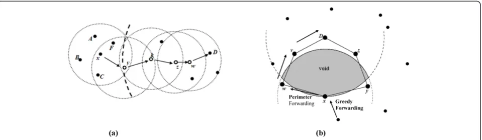
The GPSR protocol uses two forwarding strategies to route the data packet to the destination: greedy forward-ing and perimeter forwardforward-ing. In greedy forwardforward-ing, GPSR makes forwarding decisions using information about the position of immediate neighbors in the net-work topology as shown in Figure 1a. In Figure 1a, node
x wants to send a data packet destined for node D; x
sends the data packet to nodeywhich is listed inx’s list
of neighbors as shown in Table 1, and is closer to D
than any of x’s other neighbors. This greedy forwarding process is repeated by nodesy,k,z, and wuntil the data packet reaches the destination nodeD.
When the greedy forwarding strategy fails to find a neighbor closer to the destination than itself, the GPSR protocol shifts from the greedy forwarding strategy to the perimeter forwarding strategy. A simple example of
such a topology is shown in Figure 1b. Here, node xis
closer to the destination nodeD than its neighborsw
andy. Although there are two paths toD, x-y-z-Dand
x-w-v-D, xwill not choose to forward the data packet to
woryusing greedy forwarding strategy. In this case, the
GPSR protocol declares xas the local maximum to D
and the shaded region without nodes as a void region. To route the data packet around the void region, the perimeter forwarding strategy constructs a planarized graphbfor the neighbors of nodexand routes the data packet around the void region using the right-hand rule. The right-hand rule states that when arriving at nodex
from y, the next traversed edge is the one sequentially counterclockwise aboutx from edge (x, y). By applying
the right-hand rule in Figure 1b, nodex forwards the
data packet to hopw.
2.2. Related work
Several mobility prediction approaches and techniques have been proposed in the literature for MANET rout-ing protocols. The details of these approaches and tech-niques can be found in [5]. We survey here the mobility prediction research efforts in predicting the connectivity of the neighboring nodes based on the position informa-tion of the nodes.
Jia et al. [6] proposed a two-hop Hello protocol (T-Hello) aiming to improve the accuracy of the list of neighbors. By exchanging beacon packet messages within the two-hop scope, neighbor location information can be obtained, even if a neighbor has moved out of the sender’s communication range, so the corresponding entry in the neighbor tables of the nodes can be removed explicitly rather than waiting for time out. However, using two-hop hello beacon packet messages will increase the chances of beacon packets colliding with data packets and thus increase the number of retransmissions, resulting in increasing end-to-end delay and wastage of battery power [7]. Creixell and Sezaki [8] proposed a geographical routing protocol which makes routing decisions based on the current and future posi-tions of the node. To estimate the future position of the node, the authors used a prediction method based on real trajectory data. The disadvantage of this approach is in the implementation cost. The authors used single low-range laser scanners to track the pedestrian trajec-tory movements of the nodes, which necessitated a high storage space for the neighbors table because they used it to save the historical movements of the neighboring nodes.
Kai-Ten et al. [9] proposed the velocity-aided routing (VAR) protocol, which determines its data packet
routing based on the relative velocity between the intended routing node and the destination node. The VAR protocol incorporates the predictive moving beha-viors of mobile nodes in the protocol design. Xu et al. [10] proposed a mobility prediction mechanism to acquire neighborhood information at a future actual transmission time. In this prediction mechanism, the sender node will only send a request to collect informa-tion on neighbors before the transmission process, thereby conserving the energy consumption of periodical beacon packets; once the neighboring nodes receive the position request command, they will send two beacon packets at a specific interval. Based on received positions within beacon packets, the sender will predict the posi-tions of its neighboring nodes at a future transmission time. Son et al. [11] proposed two mobility prediction schemes; neighbor position prediction and destination position prediction, to overcome lost link and loop pro-blems in position-based routing protocols. The authors built their prediction schemes based on the position information of two beacon packets and the beacon time of neighboring nodes stored in the lists of neighboring nodes. Shah and Nahrstedt [12] proposed a position-delay prediction scheme which assists Quality of Service routing protocols to estimate a future instant position based on information on previous positions. Su et al. [13] proposed a simple prediction method. They calcu-lated the route expiry timeDtduring which two nodesi
andj will stay connected to each other. The same
pre-diction time approach is used by Sandulescu and Nadjm-Tehrani [14]. The authors exploited the context of mobile nodes information, such as the speed and
radio range, to estimate the contact window time tcw
between two meeting neighbors.
Cadger et al. [15] explored and analyzed the location-prediction schemes proposed in [11,12]. Both were implemented on top of the GPSR protocol. The results indicated that the addition of location prediction to
GPSR overwhelmingly improved its reliability
performance.
2.3. Limitations of current mobility prediction models
In addition to the previously observed and discussed limitations of mobility prediction models, most of the current research in mobility predictions is based on pie-cewise linear node motion between successive beacon packet updates. In addition, it assumes that the mobile nodes move at constant speed without considering direction information in the beacon packet updates or prediction techniques used. Furthermore, current research built mobility prediction models based on two or more beacon packet updates.
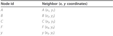
This study argues that two or more beacon packet updates are not available to the sender on its neighbors Table 1 Nodexneighbors list
Node-id Neighbor (x,ycoordinates)
A A(x1, y1)
B B(x2,y2)
C C(x3, y3)
F F(x4,y4)
list all the time for predicting a suitable node move-ment. For example, current prediction models assume the nodes have two position information points for their neighboring nodes. In some scenarios, these two points may not be available for the nodes to predict the future positions of their neighbors. For example, consider the
situation illustrated in Figure 2a, where node i moves
from positionP1 to P2. Assume that according to the
node iBPIT, nodei sends its beacon packet at position
Px. In this scenario, node Awill receive only one posi-tion informaposi-tion point from nodei. Due to this, nodeA
fails to make a prediction decision when it needs to route a data packet to destinationD.
Another limitation of current mobility prediction models is wrong prediction decisions that nodes can
make. For example, Figure 2b shows that nodeimoves
in direction d1 then changes direction at point Px to
move in direction d2. Consequently, node s received
nodei’s beacon packets at pointP1 andP2. In this
situa-tion, node s will predict that node i’s future direction will be in direction dx, while the actual direction of nodeiis in direction d2. This is because current
mobi-lity prediction models do not include the direction of movement in their prediction concept.
Based on the drawbacks observed in current mobility prediction models, this study has built a new mobility prediction model that considers the limitations described in Figure 2a, b.
3. The NWLB problem
In the GPSR protocol, every node, within a time inter-val, periodically broadcasts a beacon packet within its own transmission range. The beacon packet carries the node ID and its current position information (x,y coor-dinates). Every node that receives the beacon packet cre-ates a new entry in its list of neighbors for the incoming node beacon packet and retains this information for later use in the data packet routing process. By using the beacon packets, all the nodes in the network will
have geographical position information about their neighboring nodes.
Position-based routing protocols always route the data packet to the neighboring node closest to the destina-tion node. The sender node searches its list of neighbors for this node, but the selected next hop node may not be within the transmission range of the sender, although it is listed as a neighboring node. This is because the routing neighbor is close to the limit of the sender’s transmission range with a high probability that the
selected neighboring node may have left the sender’s
transmission range, even though it is still listed in the sender’s list of neighbors. This situation is defined as a NWLB problem.
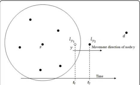
Figure 3 shows the NWLB problem; the GPSR proto-col has defined nodey at positionly1 as a routing node
since node y is clearly the neighbor closest to
destina-tiond. This is because the beacon packet heard from
nodes about nodey at timet1. However, when node s
decides to route the data packet to node y at time t2,
nodey may be in positionly2, which was not recognized
by node s at the time it made the routing decision.
Nodescan recognize that node y is no longer a
neigh-bor if it does not receive a beacon packet from it within a time interval usually greater than 3 times the BPIT [4]. At timet2, node yis out of the transmission range
of node s, but is still listed in the list of s’s neighbors (t2-t1 < 3* BPIT). This situation would let nodes route
the data packet to an out-of-date routing neighbor
(node y) and the routing data packet would be dropped
on the wireless link.
4. Effect of network parameters on the NWLB problem
Many network parameters in [16] can affect the exis-tence of the NWLB problem, including BPIT, NS,
Figure 2Limitations of current mobility prediction models
based on two position information points: (a) Only one position information point is available to nodeA.(b)Wrong prediction decision made by nodeS.
network density, node transmission range, and network area size.
4.1. Effect of BPIT and NS
One of the variables that control the node connectivity in position-based routing protocols is the node BPIT [17]. BPIT specifies the maximum time interval between the transmissions of beacon packets among the nodes. Each node in position-based routing protocols periodi-cally broadcasts beacon packets to its neighbors to make them aware of its presence (ID) and its geographical position information (x, ycoordinates). Receiving nodes, within the sender’s transmission range, create or update their neighbors list and use the information in the bea-con packets for later routing processes. Position infor-mation carried by these beacon packets becomes inaccurate as the BPIT increases. In addition, the posi-tion informaposi-tion that nodes associate with their neigh-bors in their list of neighneigh-bors becomes less accurate between beacon packets as these neighbors move.
Figure 4a depicts the effect of BPIT on NWLB in the
GPSR protocol. Here, nodes recognizes its neighboring
noden1 in its list of neighbors at position n1’ from the
beacon packet information that arrived at time t1. If
node n1 broadcasts its beacon packet, using BPIT2 at
timet3, rather than using BPIT1 at timet2, where BPIT2
> BPIT1 and t3 >t2, it is expected that there will be a
higher probability of noden1 being out of the
transmis-sion range of nodeswhich leads the NWLB problem to
be more possible to happen.
Moreover, variation of the NS means a change in the degree of node mobility which in turn affects the NWLB problem. Each node can move at different speeds and the maximum NS is the other parameter determining the occurrence of the NWLB problem. Fig-ure 4b depicts the effect of NS on the NWLB problem
in GPSR position-based routing protocols. Here, node s
recognizes its neighboring node n1 in its list of
neighbors at position n1’ at time t1. If node n1 moves
using NS1 rather than NS2, where NS2 > NS1, it is
expected that node n1will travel a greater distance and
the probability that it will be out of nodes’transmission range will increase. From Figure 4a, b, we can conclude that as the BPIT and NS increase, the NWLB problem increases.
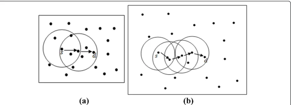
4.2. Effect of network density
The network density, which represents the number of nodes within the network area, affects the NWLB pro-blem. In MANET, the node communicates with its neighboring nodes to send, receive, and route data traf-fic. The NWLB problem is clearly evident when network density increases. Figure 5a shows the selected routing neighbor at low network density, where a small number of neighboring nodes are within the sender’s transmis-sion range, and Figure 5b shows the selected routing neighbor at high network density, where a large number of neighboring nodes are within the sender’s transmis-sion range. At low network density, the average route length (RL) to destination is about (2/3)R, where Ris the node transmission range radius. The (2/3)Rroute is more stable in routing the data packets and the routing nodes on the route are less likely to break the wireless links with their neighbors when they move. At high net-work density, the average RL to destination is closer to
R. This causes the routing nodes to be located at the
limit of the transmission range of the sender node. This route is less stable in routing the data packets and the routing nodes are more likely to break the wireless links with their neighbors in the route when they move. In addition, we observed from Figure 5a, b that a low net-work density increases the RL to the destination (num-ber of hops). In Figure 5a, the num(num-ber of hops to reach the destination is three hops, while, in contrast, high network density decreases the RL, two hops in Figure 5b.
4.3. Effect of node transmission range
The transmission range represents the limit of node connectivity with its neighbors. In the GPSR protocol,
increasing the node’s transmission range reduces the
number of hops (RL) needed to reach the intended des-tination and enhances the overall network connectivity [18]. In addition, it reduces the likelihood of the node having the NWLB problem with its neighboring nodes while they are moving. Conversely, decreasing the node’s transmission range increases the number of inter-mediate hops between the source and destination and increases the chance of the NWLB problem arising between the nodes.
Figure 6a shows the sender with a short transmission
range R1 and Figure 6b shows the sender with a long
transmission rangeR2whereR2 >R1. With a short
trans-mission range, the selected routing neighbor is closer to the sender’s transmission range limit and any routing node movement will break the wireless link with the sender. In addition to this, a short transmission range increases the RL to the destination since the data packet has to be routed using many hops before it arrives. For the long transmission range, as shown in Figure 6b, the selected routing neighbor is far from the limit of the sender’s transmission range and the probability of the
routing node movement breaking the wireless link with the sender will decrease. Moreover, the long transmis-sion range decreases the RL to the destination because the data packet is routed using fewer hops before it arrives at the destination.
4.4. Effect of network area size
Network area size represents thex andydimensions of
the network area. In the GPSR protocol, increasing the network area size yields an increment in the number of routing hops the data packet needs to use to reach the intended destination. In addition, increasing the network area size yields a decrease in the NWLB problem since the routing neighbor will be far from the limit of the sender node transmission range. Decreasing the network area size decreases the number of routing hops used to route the data packet to its destination and hence increases the average number of NWLB since the data packet will be routed to neighboring nodes closer to the limit of the sender’s transmission range.
Figure 7a, b shows a small and a large network. With a small network area, the RL to the destination is short and this increases the NWLB problem, while with a large network area, the RL to destination is long and this decreases the NWLB problem. The effect of the Figure 5Effect of network density: (a) Low network density; (b) High network density.
network area size can be considered a mirror for the network density effect explained in Figure 5. A high net-work density reflects a small netnet-work area size and vice
versa. We can create a high-density network using x
number of nodes by distributing the same number of nodes within a small network area size.
5. Proposed NWLBP model
Let us assume that the latest beacon packet was gener-ated at timet1 from neighboring node ito a particular
sender node s reporting position coordinates xi
t1,y
i t1,
velocity vi
t1, acceleration a
i
t1, and direction ∅
i
t1 such that the node i moves at an anti-clockwise angle ∅i
t1 to the horizontal. Let us also assume that the velocity vit1, acceleration ai
t1, and direction ∅
i
t1 at the instant of cur-rent timetc (the time node sdecides to forward a data
packet to i) have remained unchanged since the latest
received beacon packet time. Assume that nodeswishes
to predict the position xip,ypi of nodei at some instant
of time tc. This situation is depicted in Figure 8 and Table 2 illustrates the notations used for the NWLBP model.
From Figure 8, applying the laws of sines and cosines to the triangle KLM obtains the following formulas:
xi
xt1 and aixt1 are the speed and acceleration of
node i along the x-axis and vi
yt1 and aiyt1 are the speed
and acceleration of node ialong they-axis which can be
calculated according to the following formulas:
vi
Using Equations (1) and (2), any node can predict the future position of node iwithin its transmission range at thex-axis xi
p and the y-axis yip once the latest
posi-tion coordinates xit1,yti1, speed vit1, direction of motion
∅i
t1, and the instant of time information become avail-able to the sender node in its list of neighbors.
Figure 7Effect of network area size: (a) Small network area with sizeX1×Y1; (b) Large network area with sizeX2×Y2.
To implement the proposed NWLBP model, the nodes need to record additional position information about its neighboring nodes in their lists of neighbors. For each neighbor, the following additional data are stored: the position coordinates xi
t1,y
and the instant at time point t1 when this data are
received by the node’s list of neighbors. The node’s modified list of neighbors is shown in Figure 9.
In summary, when the sender node has a data packet to be routed to a destination, the sender first uses the position information available in its list of neighbors to predict the position of its selected routing neighbor using Equations (1) and (2). The sender node then cal-culates its distance from the predicted neighboring node position using the following formula:
Dip=
where Dip is the predicted neighboring node’s distance
from the sender node and (xs
c,ysc) is the current position
of the sender node along the xand y axes. When the
sender node finds that the value of Di
p is greater than
its transmission range, it will not route the data packet to that neighbor even though that neighbor is shown to be the closest neighbor to the destination. Using the NWLBP model, the sender node has the ability to avoid routing the data packet to a neighboring node that is
located outside the sender’s transmission range even
though it is still listed as a neighboring node.
Our NWLBP model does not contribute to any addi-tional communication overhead, intense computation, or
bandwidth use between the nodes. All the computations are done locally within the node and do not involve the neighbors participant. The NWLBP model only utilizes the GPSR protocol beacon packet to carry extra infor-mation, as shown in Figure 9, to the nodes’neighbors. Consequently, the model does not increase the number of beacon packets generated between the nodes.
6. Results and evaluation
6.1. Simulation model and assumption
In our simulation experiments, we assume the network consists of a set of wireless nodes, where each node knows its position accurately using a localization techni-que such as GPS. All nodes have the same radio range and they broadcast beacons to their neighbors, so each node is aware of its neighbors and their locations. In addition, we assume (i) nodes detect and announce accurate locations, (ii) radio ranges of all nodes are exact and symmetric, and (iii) there are no obstacles and nodes within radio range can always communicate. Admittedly, these assumptions are ideal and do not hold in practice. Violation of any of these assumptions under actual conditions can result in destruction of the GPSR protocol mechanism itself [19] as well as the prediction model. For the NWLBP prediction model, under actual conditions, as long as the node can receive a beacon packet from its neighbors, it can predict the future posi-tion of its neighbor and assist the GPSR protocol to for-ward the data packet to the best candidate neighbor in the direction of its destination.
To show the effectiveness of the NWLBP model, we built our own discrete-event simulation model using C+ + Builder 6 [20,21]. The simplicity of the GPSR protocol and NWLBP model implementation made us the confi-dent that our simulation model compared well with other simulation tools such as NS2 [22]. NS2 places more emphasis on the performance and validity of a dis-tributed protocol than on the visual or real-time visibi-lity features of the simulation. In addition, NS2 has a high consumption of computational resources and lacks a generalized analysis tool. Figure 10 shows a set of screen snapshots for our implementation of the GPSR protocol and an illustration of the NWLB problem. Table 2 Notations for NWLBP model
Variables Definition
t1 Instant time point of node position
(xi
t1 The node direction with respect tox-axis
tc Instant time point of current time
(xip,yip) The predicted position of nodeiat timetc
The data points presented in the simulation results were calculated as the average of ten simulation runs to eliminate the effect of any anomalous individual result because we observed a realistic variance among the points using ten or more simulation runs. We plotted the 95% confidence interval as error bars on the figures.
Our simulation study was conducted with varying numbers of nodes, numbers of data traffic sources, and NSs. We simulated 50, 60, 70, 80, 90, and 100 nodes, 5, 10, 15, 20, 25, and 30 data traffic sources. NSs are uni-formly distributed between 0 and maximum speed of 5, 10, 15, 20, 25, 30, 35, and 40 m/s, keeping all other simulation parameters in Table 3 as constant unless otherwise stated. The source and destination nodes were randomly selected from the nodes in the simulation sce-nario. The GPSR protocol is used as the underlying routing platform protocol.
The performance metrics used in simulation experi-ments are
1. Control overhead: The control overhead metric represents the total number of beacon packets exchanged by all the nodes in the network.
2.End-to-End delay: This metric represents the aver-age end-to-end delays experienced by each data packet at each hop on its way from source node to destination node.
3.Non-optimal route:This metric represents the num-ber of hops experienced by each data packet along its route from source node to destination while it passes through the intermediate nodes.
4.Node false position:The node false position metric represents the difference in distance in meters between the real (accurate) and the false (inaccurate) neighboring nodeiposition in the nodejlist of neighbors.
In this study, we used the bound simulation area (BSA) mobility model [23] as the pattern for the movement of nodes as shown in Figure 11. Unlike other mobility models such as the random way point mobility model [23], the BSA mobility model reflects
the relationship between the mobile nodes’ previous
and current motion behavior. In BSA, speed and direction of current movement randomly diverge from the previous speed and direction after each time incre-ment. This makes the movement of the nodes smooth in both speed and direction. The position, speed, and direction of movement of the nodes are updated at
every Δttime step according to the following
formu-las:
v(t+t)=min[max(v(t)+v, 0),vmax] (8)
∅(t+t)=∅(t)+∅ (9)
x(t+t)=x(t)+v(t)×COS∅(t) (10)
y(t+t)=y(t)+v(t)×SIN∅(t) (11)
where vmax is the maximum speed defined in the
simulation,Δvis the change in speed which is uniformly distributed between [-Amax ×Δt, Amax ×Δt,],Amax is
the maximum acceleration of a given mobile node,Δ∅
is the change in direction which is uniformly distributed Figure 10GPSR protocol implementation: (a) Greedy and perimeter forwarding strategies.(b)NWLB problem;9ais the position of node 9 recognized in the SRC 0 list of neighbors;9bis the position of node 9 at the instance in time of the packet forwarding decision made by SRC 0 toward DST 0.
Table 3 Simulation parameters
Description Value Unit
Simulation time 1200 s
Network area size 1000 × 1000 m2
Maximum node speed 40 m/s
Maximum acceleration 10 m/s2
Maximum angular change 90 degree
Updating time steps (Δt) 1000 millisecond
Node transmission range 250 m
Data traffic (CBR) 5 packets/s
No of data traffic sources 5 sources
Beacon packet interval-time 3 second
Bandwidth 2 mbps
Data packet size 512 bytes
Beacon packet size 64 bytes
-between [-∞ × Δt, ∞ × Δt], and ∞ is the maximum angular change in the direction of mobile node travel.
6.2. Effect of network parameters on the NWLB problem
Figure 12 shows the effect of BPIT and NS on the occurrence of the NWLB problem in the GPSR protocol for different BPIT and NS values. As the BPIT and NS increase, the percentage of neighbors who break the wireless link with the sender also increases. Longer BPIT and a high NS yield results in neighbors being listed in the sender’s list of neighbors when they are in fact outside the transmission range as shown in Figure 4.
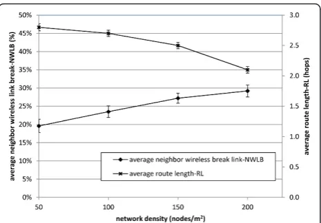
Figure 13 shows the effect of network density on the
percentage of NWLB observed in the sender’s list of
neighbors and the average RL for four different network densities as shown in Table 4. In general and for the reasons shown in Figure 5, when the network density
increases, the average NWLB increases while the average RL decreases.
Figure 14 shows the effect of transmission range on the average NWLB and average RL. As shown in Figure 6, when the transmission range increases, the chance of the selected forwarding neighbor being at the limit of the transmission range will reduce, which results in fewer wireless link breakages with the sender. In addi-tion, a longer transmission range decreases the RL since the packet has to be routed using fewer intermediate hops.
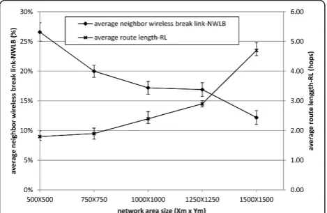
Figure 15 shows the effect of network area size on the average NWLB and average RL. As shown in Figure 7, when the network area size increases, the average NWLB decreases while the average RL increases. The increment in the network area size results in an increase in the number of routing hops between the source and destination nodes. With more hops between the source and destination, it is expected to get greater RL between them. Both the network density and network area size have the reverse effect on the average NWLB and aver-age RL. Increasing the network area has the same effect of decreasing the network density on the average NWLB and the inverse effect on the average RL as shown in Figure 13. In other words, when we distribute the nodes within a small network area size, we increase its density and when we distribute the nodes within large network area size, we decrease the nodes density within it. Figure 11BSA mobility model.
Figure 12Percentage of NWLB versus NS and BPIT.
Figure 13Effect of network density on average NWLB and
average RL.
Table 4 Nodes versus network density
Nodes Network density (nodes/m2)
50 0.00005
100 0.00010
150 0.00015
6.3. WNLBP model results and evaluation 6.3.1. Control overhead
Throughout our simulation experiments, we observed that the overheads of the beacon packets remained unaf-fected during the change in NS setting values in the GPSR protocol with and without the use of the NWLBP model. The beacon packets were not affected by NS. Increasing the NS did not result in a corresponding increase in the number of beacon packets in the basic mechanism of the GPSR protocol or in the implementa-tion of the NWLBP model. The same observaimplementa-tion applied to the effect of the number of data traffic sources. Figure 16 shows that the increase in the num-ber of the nodes increases the overhead for the control packets. Extra nodes in the network mean that extra beacon packets will be broadcasted by each node. 6.3.2. End-to-end delay
Figure 17 shows the average end-to-end delay in the GPSR protocol with and without using the NWLBP model as a function of NS. Using the NWLBP model
achieves a lower average end-to-end delay compared to the GPSR performance without using the NWLBP model, because NWLB problem causes the data packet to be retransmitted several times to the neighboring node that is listed in the sender’s list of neighbors but is out of the its transmission range. The data packet retransmission causes additional delays at the intermedi-ate nodes. However, using the NWLBP model, the sen-der routes the data packet to the listed routing neighbor that is within the sender’s transmission range. Conse-quently, the data packet avoids additional delays on its route to its destination.
Figure 18 shows the average end-to-end delay as a function of the number of nodes. In general, as the number of nodes increases, the average end-to-end delay increases because of the effect of node density in the network as shown in Figure 5, which is caused by
Figure 14Effect of transmission range on average NWLB and
average RL.
Figure 15Effect of network area size on average NWLB and
average RL.
Figure 16Control overhead versus number of nodes.
Figure 17Average end-to-end delay versus maximum node
many occurrences of the NWLB problem. Using the NWLBP model achieves less average end-to-end delay even though the number of nodes increases in the net-work. This is because the NWLB model guarantees to route the data packet to the neighbor listed in the sen-der’s list of neighbors and within its transmission range.
Figure 19 shows the average end-to-end delay as a function of the number of data traffic sources in the network. It can be seen that as the number of data traf-fic sources increases, the average end-to-end delay also increases. The increase in the number of data traffic sources in the network causes more data packets to be rerouted using different paths and hence to be subjected to the NWLB problem. Using the NWLBP model achieves less average end-to-end delay due to its mechanism of routing the data packets to a neighbor within the sender’s transmission range.
6.3.3. Non-optimal route
Figure 20 shows the non-optimal route in the GPSR protocol, using and without using the NWLBP model, as a function of the NS in the network. In general, as the NS increases, the non-optimal route also increases. The high speed increases the possibility of out-of-date position information in the senders’ list of neighbors which leads to a high possibility of choosing the wrong neighboring node for data packet routing. Using the NWLBP model achieves better (fewer) non-optimal routes. This is because the network topology informa-tion is maintained by the NWLBP model which yields more accurate position information and more suitable selection of the routing neighbor from the sender’s list of neighbors.
Figure 21 shows the non-optimal route in the GPSR protocol, using and without using the NWLBP model, as a function of the number of nodes in the network. We note that as the number of nodes increases, the non-optimal route decreases. This is because of the effect of network density as shown in Figure 5. When the number of nodes increases in the network, the sen-der node has many candidate neighbors on its list for routing the data packet. This reduces the chance of wrong selection in picking the neighbors on the list but
out of the sender’s transmission range. The NWLBP
model performs better in reducing the non-optimal routes because of better decisions in picking the routing neighbor from the sender’s list of neighbors.
Figure 22 shows the non-optimal route in the GPSR protocol, using and without using the NWLBP model, as a function of the number of data traffic sources in the network. As the number increases, the number of optimal routes increases. The increase in the non-optimal route is due to more source-destination data
Figure 18Average end-to-end delay versus number of nodes.
Figure 19Average end-to-end delay versus number of data
flows, which cause a high rate of data packets to be rou-ted to a neighbor out of the sender’s transmission range. The NWLBP model performs better on non-optimal routes due to the NWLBP model mechanism for routing
the data packet to the neighbor within the sender’s
transmission range. 6.3.4. Node false position
Figure 23 shows the node false position in the GPSR protocol, using and without using the NWLBP model, as a function of the NS. In general, as the NS increases, the number of false positions increases due to the effect of NS, as shown in Figure 4. Figure 23 shows that the NWLBP model reduces the number of node false posi-tions for all NSs because accurate node position infor-mation is maintained in the senders’list of neighbors.
Figure 24 shows the node false position in the GPSR protocol, using and without using the NWLBP model,
as a function of the number of nodes. In both cases, as the number of nodes increases, the number of node false positions also increases since there are more nodes in the network with more inaccuracies in their position information. Figure 24 shows that the NWLBP model achieves fewer node false positions. We did not observe any influence of the number of data traffic sources on the number of node false positions. As the number of data traffic sources increases, the node false position remains static since a node false position is not related to the number of data traffic sources in the network. We observed that the increase in the number of data traffic sources does not affect the distance between the actual and false node positions.
7. Conclusion and future work
In this study, we introduced the NWLB problem between the sender node and its routing neighboring
Figure 21Non-optimal route versus number of nodes.
Figure 22 Non-optimal route versus number of data traffic
sources.
Figure 23Node false position versus maximum node speed.
node in the GPSR position-based routing protocol. In addition, we introduced the BPIT, NSnode speed, net-work density, node transmission range, and netnet-work area size as network parameters that can affect the occurrence of this problem. To overcome the NWLB problem, we proposed the NWBLP model, which helps the sender to predict the position of the routing neigh-boring node before routing the data packet to it. The NWLBP model helps the sender make an accurate pre-diction based on up-to-date and accurate position infor-mation. The simulation results show that the NWBLP model achieved a better network performance for differ-ent performance metrics such as control overhead, end-to-end delay, non-optimal route, and node false position. In future work, we aim to show that the NWBLP model can support many position-based routing proto-cols. Some perform better in a mobile network with high mobility, while others perform better in a mobile network with low mobility. A possible area of future research could be to examine the NWBLP model under more realistic conditions such as position estimation error and obstacle environment. In addition, the perfor-mance of the NWBLP model would be an interesting study when applied in the real MANET environment since it is easy to implement. Moreover, the NWBLP model may be affected if the node changes its direction of motion, speed, or acceleration value after broadcast-ing its last beacon packet and before its next scheduled beacon packet, based on its BPIT. Furthermore, consid-ering the error in node-predicted position when apply-ing the NWBLP model would be an interestapply-ing future study since the error in the predicted node position can be investigated if the mobility pattern of the nodes is known.
Endnotes
a
Wireless link refers to the communication channel
between two neighboring nodes. bA planar graph is a
graph that can be drawn in the plane with no crossing edges.
Abbreviations
BPIT: beacon packet interval-time; BSA: bound simulation area; CBR: constant bit rate; DREAM: distance routing effect algorithm for mobility; GPS: global position system; GPSR: greedy perimeter stateless routing; LAR: location aided routing; MANET: mobile ad hoc network; NS: node speed; NWLB: neighbor wireless link break; NWLBP: neighbor wireless link break prediction; RL: route length; VAR: velocity-aided routing.
Acknowledgements
This study was supported in part by the Centre for Research and
Instrumentation Management (CRIM), University Kebangsaan Malaysia (UKM), Malaysia (Grant UKM-GGMP-ICT-035-2011).
Author details
1
School of Computer Science, Faculty of Information Science and
Technology, University Kebangsaan Malaysia, 43600 Bangi, Selangor, Malaysia
2Department of Computer Engineering, Faculty of Engineering and
Technology, The University of Jordan, 11942, Amman, Jordan
Competing interests
The authors declare that they have no competing interests.
Received: 5 July 2011 Accepted: 16 May 2012 Published: 16 May 2012
References
1. M Mauve, J Widmer, H Hartenstein, A survey on position-based routing in mobile ad hoc networks. IEEE Netw.15(6), 30–39 (2001). doi:10.1109/ 65.967595
2. DK Elliott,Understanding GPS: Principles and Applications, 2nd edn. (Artech House Publishers, London, 2005)
3. SJ Philip,Scalable Location Management for Geographical Routing in Mobile Ad Hoc Networks, (The State University of New York, Buffalo, 2005) 4. B Karp, HT Kung, GPSR: Greedy Perimeter Stateless Routing for wireless
networks, inProceedings of the Sixth Annual International Conference on Mobile Computing and Networking (MOBICOM 2000), pp. 243–254 (2000) 5. D Gavalas, C Konstantopoulos, B Mamalis, G Pantziou, Mobility prediction in
mobile ad-hoc networks, inNext Generation Mobile Networks and Ubiquitous Computing, ed. by Pierre S IGI Global, Hershey, pp. 226–2406 (2011) 6. Y Jia, W Ying-you, Z Hong, A solution to outdated neighbor problem in
wireless sensor networks, inProceedings of 3rd IEEE International Conference on Computer Science and Information Technology (ICCSIT2010), pp. 277–280 (2010)
7. W Ye, J Heidemann, D Estrin, An energy-efficient MAC protocol for wireless sensor networks, inProceedings Twenty-First Annual Joint Conference of the IEEE Computer and Communications Societies (INFOCOM 2002).3, 1567–1576 (2002)
8. W Creixell, K Sezaki, Routing protocol for ad hoc mobile networks using mobility prediction. Int J Ad Hoc Ubiquit Comput.2(3), 149–156 (2007). doi:10.1504/IJAHUC.2007.012416
9. F Kai-Ten, H Chung-Hsien, L Tse-En, Velocity-assisted predictive mobility and location-aware routing protocols for mobile ad hoc networks. IEEE Trans Veh Technol.57(1), 448–464 (2008)
10. H Xu, M Jeon, S Lei, J Cho, S Lee, Localized broadcast oriented protocols with mobility prediction for mobile ad hoc networks, inProceedings of Next Generation Teletraffic and Wired/Wireless Advanced Networking340–352. 4003/2006
11. D Son, A Helmy, B Krishnamachari, The effect of mobility-induced location errors on geographic routing in mobile ad hoc sensor networks: analysis and improvement using mobility prediction. IEEE Trans Mob Comput.3(3), 233–245 (2004). doi:10.1109/TMC.2004.28
12. SH Shah, K Nahrstedt, Predictive location-based QoS routing in mobile ad hoc networks. Proceeding of IEEE International Conference on
Communications (ICC2002).2, 1022–1027 (2002)
13. W Su, S Lee, M Gerla, Mobility prediction and routing in ad hoc wireless networks. Int J Netw Manag.11(1), 3–30 (2001). doi:10.1002/nem.386 14. G Sandulescu, S Nadjm-Tehrani, Adding redundancy to replication in
window-aware delay-tolerant routing. J Commun (Special Issue in Delay Tolerant Networks, Architecture, and Applications).5(2), 117–129 (2010) 15. F Cadger, K Curran, J Santos, S Moffett, An analysis of the effects of
intelligent location prediction algorithms on greedy geographic routing in Mobile Ad-Hoc Networks, inProceedings of the 22nd Irish Conference on Artificial Intelligence and Cognitive Science, (University of Ulster AICS 2011, Derry, Northern Ireland, 2011)
16. J Tsumochi, K Masayama, H Uehara, M Yokoyama, Impact of mobility metric on routing protocols for1 Mobile Ad Hoc Networks, inIEEE Pacific Rim Conference on Communication, Computers and Signal Processing (PACRIM 2003).1, 322–325 (2002)
17. ID Chakeres, EM Belding-Royer, The utility of hello messages for determining link connectivity, inThe 5th International Symposium on Wireless Personal Multimedia Communications.2, 504–508 (2002) 18. J Gomez, AT Campbell, A case for variable-range transmission power
control in wireless multihop networks, inProceeding of Twenty-third Annual Joint Conference of the IEEE Computer and Communications Societies (INFOCOM2004).2, 1425–1436 (2004)
20. C++Builder 6 http://www.embarcadero.com/products/cbuilder 21. R Saqour, M Ismail, M Shanudin, Discrete-event simulation modeling tool
for routing process in GPSR ad hoc network routing protocol, in Proceedings of IEEE International Conference on Telecommunications and Malaysia International Conference on Communications (ICT-MICC 2007), pp. 86–90 (2007)
22. Network Simulator 2 (ns-2) http://isi.edu/nsnam/ns/
23. T Camp, J Boleng, V Davies, A survey of mobility models for ad hoc network research, inWirel Commun Mob Comput (WCMC) (Special issue on Mobile Ad Hoc Networking: Research, Trends and Applications).2(5), 483–502 (2002)
doi:10.1186/1687-1499-2012-171
Cite this article as:Alsaqouret al.:Effect of network parameters on
neighbor wireless link breaks in GPSR protocol and enhancement using mobility prediction model.EURASIP Journal on Wireless Communications and Networking20122012:171.
Submit your manuscript to a
journal and benefi t from:
7Convenient online submission
7Rigorous peer review
7Immediate publication on acceptance
7Open access: articles freely available online
7High visibility within the fi eld
7Retaining the copyright to your article