R E S E A R C H
Open Access
available at the end of the articleAbstract
In this paper, we develop a multi-model adaptive control strategy to be applied on delay compensation schemes for stable/unstable LTI MIMO systems. The only requirement is that the delay should be bounded and decoupled from the control strategy. The delay identification problem is formulated as an optimization one, and it is framed on the abstract definition of the Generalized Pattern Search Method (GPSM). Taking advantage of the global convergence analysis presented by GPSM, we make a stability analysis of the proposed approach and delay identification
capabilities. Simulation examples show the usefulness of the proposed strategy proving that the scheme is capable of identifying the delay and stabilizing the system even with a larger delay. The capabilities of the approach are tested on a
second-order delayed unstable process, a MIMO unstable systems and an irrigation channel model. Additionally, simulation examples on an irrigation channel with time-varying delay are presented.
1 Introduction
The external delay in a process causes the output signal to be delayed with respect to the input. If a control strategy has to be designed for this system, the presence of the delay makes it a more difficult task, especially, when the rational part of the system is unstable [, ]. Various strategies have been used to counteract the delay effect. Thus, the tuning of PID controllers is perhaps the most widely used. In [–], different tuning rules for stable/unstable systems with delay can be found. The disadvantage of such techniques is that they only work well, when the delay is small compared with the time constant of the system [].
For systems, where the delay is dominant (i.e., the delay is big compared with the time constant of the system), different control strategies such as delay compensation schemes (DCS) should be used, being the most well-known the Smith predictor and its modifica-tions for unstable and integrative systems [–]. Generally, these approaches have to be applied offline to the nominal parameters of the system known beforehand. An additional shortcoming is the lack of robustness to small uncertainties in the delay. In practice, when using a DCS for an unstable system, it is very difficult to ensure the closed-loop stability in the presence of delay uncertainty. This makes the DCS design considerably more difficult than its stable counterpart. In this way, much effort has been dedicated during the last years to the design of controllers for systems with delay uncertainty.
Recently, a framework focused on the identification and control of systems with delay uncertainty, has been proposed both for stable [–] and integrative [] systems. The approach presented is based on the classical SP and a model scheme. The multi-model scheme contains a battery of time-varying multi-models which are updated using a mod-ification rule. Each model possesses the same rational component but a different delay value. The algorithm compares the mismatch between the actual system and each model and selects, at each time interval, the one that best describes the behaviour of the ac-tual system, providing online identification of the delay while simultaneously ensuring the closed-loop stability. The way in which the delay varies is determined by a heuristic optimization; this allows both the delay identification and the system control. Addition-ally, this approach leads to a robustly stable closed-loop system while achieving a great performance for systems with unknown long delays.
In this sense, the work presented in [] is extended in this paper to potentially un-stable and integrative systems. In this case, the control scheme is based on the modified Smith predictor (MoSP) introduced in [], and the optimization is framed into a Pattern Search Method (PSM) []. It is worth emphasizing that the component by component delay identification in an unstable MIMO system is a difficult task, since it is impractical to estimate from open-loop experiments.
Control-oriented model identification methods have been of great interest in the pro-cess control community, and there are different approaches, such as design of optimal controllers, based on the particle swarm optimization [], LMI optimization [–] to treat the identification problem. The drawback of all these works is that the optimization is done offline. Recently, a systematic closed-loop parametric online identification method based on a step response test and online weight least squares optimization was proposed in [] for integrative and unstable processes. However, this work is treated without dealing the control strategy. Therefore, the modification of controller parameters must be done offline.
In this paper, the delay identification is formulated as an optimization problem, which is solved using the so-called Pattern Search Method (PSM). The PSM has been used in math-ematics and optimization theory [, ], but its use in control is rather limited, with few works on it, [, ]. Moreover, in these two works, there is neither an analysis of conver-gence nor a frame on the PSM. This contrasts with the present work, where the proposed PSM is framed correctly on the generalized PSM [], and therefore, the proposed PSM inherits the general convergence properties. Thus, analytical stability properties are for-mulated for this approach adequately and easily, since previous results and concepts can be used for this purpose.
The proposed approach is tested on different systems models and under different con-ditions as: a second-order delayed unstable process, where an uncertainty in the rational component of the system is taken into account; also it is tested on a MIMO unstable sys-tems and on an irrigation channel model, which is an integrative MIMO system. Addition-ally, simulation results have been extended to time-varying ones showing the potential and applications of the proposed approach.
The paper is organized as follows. Section states the problem formulation. Section presents the proposed control scheme framed on the GPSM. The stability analysis is per-formed in Section . Simulation examples are presented in Section . Finally, Section summarizes the main conclusions.
2 Problem formulation
Let us consider the following MIMO transfer function model:
G(s) =Gdfij(s)e–hijs=Gdfij(s)•e–hijs
=Gdf(s)•H(s), ()
whereGdf(s) is a matrix containing the rational component of the system,H(s) = (Hij(s)) = (e–hijs), fori,j= , , . . . ,n, is a matrix containing only delays, and•denotes the Schur (or component-wise) product []. The following assumptions are made about system ().
Assumption The rational transfer function matrixGdf(s) is proper, with no pole-zero unstable cancellations and known.
Assumption The delay between each input/output component lies in a known compact
interval. That is, there exist two known matricesH= (hij),H= (hij)∈Rn×nsuch thath ij≤ hij≤hij,∀i,j.
Assumption is feasible in many control problems, where a nominal model of the system is available beforehand, and it does not posses unstable pole-zero cancellations. However, the delay may be unknown or even time-varying, and hence it has to be estimated []. Note that there is no assumption on the stability ofGdf(s) being potentially unstable. As-sumption will be used in the proposed pattern-search-based algorithm to estimate the delay in Section , and it is feasible in many practical control problems, where bounds on the delay are known.
2.1 Modified Smith predictor
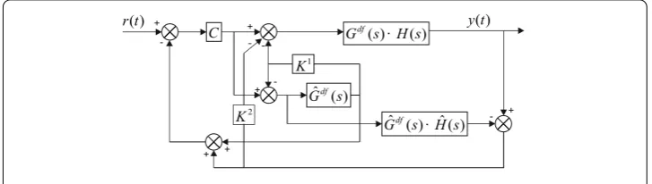
The MoSP [] is shown in Figure . Gˆdf(s)• ˆH and Gdf(s)•H are the transfer func-tions of the plant model and the actual plant, respectively. This structure has three con-trollers which are designed for different objectives. CompensatorK =diag(K
Figure 1 Modified Smith predictor structure.
We omit by notation simplicity the arguments, in the next equations. Thus, the Laplace transform with zero initial conditions of the closed-loop response obtained from Figure is given by
Y=Gdf •HI+K+CGˆdf –CGˆdf • ˆHχˆ–χ+CGdf •H–CR, () where χ= (I+K(Gdf •H)),χˆ = (I+K(Gˆdf • ˆH)). If Assumption holds (the model perfectly matches the plantGˆdf(s) =Gdf(s)) andHˆ =H, then () reduces to the simplified transfer function
Y=Gdf •HI+K+CGdf–CR. ()
Hence, the system with internal delay that appears in Eq. (), becomes a system with ex-ternal delay in Eq. (). Therefore, this is precisely a topology that decouples the delay from the control strategy, making the system easier to control, since compensatorsK,Kand Care designed regardless of the delay (i.e., based only on the rational component of the system which is known beforehand). Otherwise, if the delay is not known beforehand, the exact compensation cannot be performed despite that the rational component is known, and the closed-loop Eq. () can be potentially unstable.
The problem faced corresponds to the case when the matrix delayHis unknown, and our objective is to obtain an estimation of the matrix delayHˆ to be used in the MoSP struc-ture depicted in Figure in order to guarantee the stability of the system. The method of estimating the delay involves the formulation of the identification problem as an optimiza-tion problem solved online by PSM, which is briefly explained below.
2.2 Generalized pattern search method (GPSM)
GPSM was proposed in [] for derivative-free unconstrained optimization (minimization in this case) of continuously differentiable convex functionsJ:Rn→R.
The GPSM consists of a sequence of iterationsHˆknom,k∈N. At each iteration, a num-ber oftrial stepshn
kare added to the iterationHˆknomto obtain a number oftrial points ˆ
Hn
k =Hˆknom+hnkat iterationk. The objective functionJis evaluated on these trial points through a series ofexploratory moves, which defines a procedure in which the trial points are evaluated, and the values obtained are compared withJ(Hˆnom
k ). Then the trial steph∗k associated with minimum value ofJ(Hˆnom
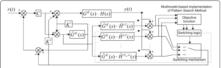
Figure 2 Basic architecture (based on MoPS) of the control scheme.
on the value ofhnk–. The evolution of the trial points establishes the convergence prop-erties of the algorithm. A full PSM explanation can be found in [].
3 Proposed control scheme using PSM
The basic structure of the proposed scheme is depicted in Figure . The MoSP and the PSM are complemented with four elements: a set of trial points, an objective function for evaluating the potential behaviour of each model, a switching logic, which monitors the index periodically and decides the best model to be used in the control law, and the switching mechanism, which is intended to reduce the possible mismatch between the nominal and the actual output of the system. The following subsections consider in detail the different elements of the proposed architecture and how they fit into the GPSM.
3.1 The patterns
The proposed architecture is composed of patterns, which are directions in the search space starting from the nominal delayHˆk= (hˆkij)∈Rn×n. The patterns are modified at each iteration to obtain a new set of trial points. These trial points are time-varying and automatically adjusted by the algorithm as corresponds to the PSM framework. The trial steps are defined by
hp,lk =BlkCp,l, ()
wherehp,lk ∈Rn×n, forp= , , . . . ,Nmandl= , , . . . ,n, whereNmis the number of mod-els (Nmshould be odd, since the nominal model should always be evaluated), the basis vec-torBl∈Rn×(vector having one in the positionlth and zeros elsewhere), the step length parameter,k= [hk,hk, . . . ,h
Nm
k ]T∈R×Nm, is adjusted by the algorithm whose val-ues are defined initially by the designer and the constant matrixCp,l∈RNm×n(matrices having one in the position (lth, pth) and zeros elsewhere). In such a way that the trial points take the form ()-().
ˆ
Hk,,Hˆk,, . . . ,HˆkNm,=Hˆk+h,k ,Hˆk+hk,, . . . ,Hˆk+hNm,k
()
ˆ
Hk,,Hˆk,, . . . ,HˆkNm,=Hˆk+h,k ,Hˆk+hk,, . . . ,Hˆk+hNm,k
()
.. .
ˆ
Hk,n,Hˆk,n, . . . ,HˆkNm,n=Hˆk+h,nk ,Hˆk+hk,n, . . . ,Hˆk+hNm,nk
It can be seen that the trial points are generated by the addition of the patterns, which in turn are generated by the length parameterk, to the nominal modelHkˆ . Note that the zero state (no changes in the nominal model) and both positive and negative directions to changeHˆkshould all be included, as explained in the definition ofkin Section .. In this way, it is ensured that all the search space is evaluated.
3.2 Objective function
The second element of the proposed scheme is an objective function aimed at evaluating the behavior of all the trial pointsHˆk(p,l). The suggested objective function is
J(p,l)Hˆ(p,l),t= does (). This dependence is expressed in () implicitly as dependence witht.Tresis the so-called residence time and defines the time interval window, where the delay modelHˆ(p,l) is evaluated. Also it can be seen that the objective function () differs from the proposed in [], because it is time-dependent. However, it is not a problem to frame the present approach into the GPSM as explained in Section ..
The Laplace transform of the output error,e(p,l)with zero initial conditions is given by
E(p,l)=GdfH–Hˆ(p,l)χˆ–χ–CR, () where= ((I+ (K+C)Gˆdf –CGˆdf • ˆH(p,l))χˆ–χ+CGdf •H). It is readily seen from () that the error is zero whenHˆ(p,l)=H. According to this fact, the search for the minimum of the function () leads to an estimation of the actual matrix delay. Thus, the identifica-tion problem is converted into an optimizaidentifica-tion one. It is important to notice that () is a continuously differentiable function, since it is defined as the square of the subtraction of two functions that are continuously differentiable. Also, () satisfies the compactness con-dition stated in []. On the other hand, the simple decrease concon-dition (convexity) cannot be guaranteed to be satisfied.
3.3 Proposed pattern search method
The PSM monitors at time instants being integer multiple of the residence time the ob-jective function and selects the nominal delay, which is the best estimation of the actual one. The nominal delay is used within each time interval to generate the control law. The initial trial point is selected by the designer asHˆnom
k= andk=using Assumption . From this moment onwards, the PSM can be formally expressed as the Algorithm .
The trial points ()-() are compared (line of Algorithm ) with nominal model using the performance index (). In this way, the element associated with the lowest value of the objective function is obtained, and this represents the best delay. Next, the new trial points are generated based onk, which is given by
Algorithm MIMO delay identification based on PSM.
: fort> do{At multiples of the residence time.}
: ift=wTres,w∈Nthen
where the reduction factor matrix is given by
k=ηk ()
for <η< . Furthermore,limk→∞k= . Notice that sincek contains positive and negative values, the trial points () and () are defined as additions and subtractions to the nominal model. These positive and negative values along with the zero value in the central position of () and an adequate value forNmandallow to make a dense search in the delay space (i.e., the complete search space can be explored to find the minimum of the objective function ()).
The models are not equally spaced in the delay space since the mesh is more refined near the nominal delay. To show this issue, the separation between consecutive patterns can be calculated according to Eq. (). Thus, consider only the positive values fork(since the
separation for the negative part is identical due to symmetry):k= [lk] l=(Nm–) l= . Then, the separation between two consecutive patterns is:δk= (l+ )k–lk= (l+ )k withl= , , . . . , (Nm– ) – . Notice thatδkincreases aslincreases, which means that the patterns are more separated as they get far from the nominal model. The largest separation between patterns is given byδk,max= (Nm– )k, while the minimum separation is given byδk,min=kat each iteration,k.
3.4 Convergence results of the identification scheme
This section states the convergence results for the Algorithm , which guarantee the iden-tification of the actual matrix delay. The proof is divided into two steps. Firstly, the condi-tions under which () has a unique global minimum whenHˆnom
k =Hare stated. Secondly, it will be shown that the proposed Algorithm is able to asymptotically find the global minimum of functionJ(Hˆ,t).
From (), it can be seen thatJ(Hˆ,t) = whenHˆ =H, andJ(Hˆ,t)≥ since its integrand is non-negative. Thus, the global minimum is calculated whenJ(Hˆ,t) = . The next As-sumption will be used subsequently.
Assumption Fix an arbitraryTres> . The reference signalsr(t),r(t), . . . ,rn(t) satisfy the following conditions:
ri(t)=ri(t–λ) ()
and
ri(t–γi) –ri(t–λi)= – n
j=,j=i
j
rj(t–γj) –rj(t–λj)
()
for allλ,λi,γi∈[h,h]∩(,∞) fori= , , . . . ,n,h=maxhij,h=minhij,j=i,j∈ {, }and t∈I⊆[kTres, (k+ )Tres),k∈N, for at least one connected intervalIof positive measure.
The meaning and role played by Assumption in the delay identification is pointed out in the proof of Lemma . Basically, the interpretation of () is that the reference signals cannot be periodic, and that the different sums between them cannot be equal to other ref-erence signal or a delayed version of it. This interpretation allows us to generate refref-erence signals easily in practice despite Eq. () looks complicated.
Lemma The function()has a unique global minimum atHˆ =H for all t≥,provided that the reference signals r(t),r(t), . . . ,rn(t)satisfy Assumptionfor a given Tres> .
Proof The proof is done in the same way as the proof of Lemma in [].
In conclusion, if compensation between the different components is not possible due to Assumption , then the actual matrix delay is the unique global minimum for the objective function ().
Lemma states that the minimum ofJ(Hˆ,t) is unique if the reference signalsrj(t) satisfy Assumption . The approach presents the peculiarity that the global minimum is always the same, but for each time window, the functionJ(Hˆ,t) may take a different form. How-ever, the same ideas and concepts from the GPSM can still be applied to this problem.
search into dense, according to the ideas in [], which can be achieved in the presented algorithm making the parametervery close to zero andNmsufficiently large.
Now, we can formulate the following result on delay identification based on the dense construction of patterns according to the ideas in [] and the global convergence results stated in [].
Theorem Consider the delay system given by()satisfying Assumptionsand.Thus, the PSM based Algorithmthrough models()-()can identify the actual matrix delay provided that the reference signals r(t),r(t), . . . ,rn(t)satisfy Assumptionfor a value of Tres,is sufficiently close to zero and Nmis sufficiently large.
The proof of Theorem relies on two basic features. The first one is that the mesh gen-erated by the patterns is dense in the search space. This fact allows obtaining an estimate of the delay lying in a neighbourhood of the actual delay, where there is no local optimum except the global one. Secondly, the algorithm is proven to converge to the actual delay by reduction to the absurd.
Proof If the initial estimate is the actual matrix delay, then the delay is identified and the theorem is proven. Thus, consider thatHˆ =H. The particular problem of pattern search methods is that the objective function to be optimized is time-varying, since it changes at each residence time. In this way, we may consider each of the objective func-tions () evaluated at each residence time multiple,t=kTres, to define the family of func-tions,Jk(Hˆ) =(k–)Trest=kTres (y(τ) –yˆ(τ,Hˆ))dτ, which satisfy thatJk(Hˆ) = if and only ifHˆ =H. Lemma ensures that all these functions possess a common unique global minimum pro-vided that Assumption holds. However, each of these functions may possess a number of local minima.
Thus, one of the following two cases will arise:
(a) All the functionsJk(Hˆ)only have the actual matrix delay as local minimum. Then, any new iterationHˆbelongs to an interval, where there is no other minimum than
the actual delay. This would be the best situation since the optimization process will not be threatened by the presence of local minima.
(b) At least one of the functionsJk(Hˆ)has extra local minima being distinct of the
global minimum. In this case, let us denote byK⊆Nthe set indexing the functions having local minima andCk, withk∈K, the set of all delays being local minima of
functionJk(Hˆ), excluding the global optimum at the actual matrix delay. Hence,Jk(Hˆ) > for allHˆ ∈Ckand allk∈K. Moreover, we can define
θ=inf{Jk(Hˆ)| ˆH∈Ck,k∈K}> which exists and is finite and positive. The
parameterθdefines a neighbourhood,I, around the actual delay, where all the functionsJk(Hˆ)do not have any local minima except the global one. In addition, denote byλthe diameter of the setI. Thus, if the patterns define a dense subset of the search space in such a way that the patterns cover all the space,
(Nm– )
≥H–H(i.e., the spread of the patterns given by the total amplitude of
is larger than the uncertainty range given by Assumption ), and the separation
between them is sufficiently small,δ,max= (Nm– )<λ, which is achieved
with a sufficiently largeNmand a sufficiently small, then for any initial
iteration provides an estimate within a neighbourhoodIof the actual matrix delay, where all the functions do not have any other minimum than the actual one.
In conclusion, the iterationHˆ is always guaranteed to belong to an interval, where the actual matrix delay,H, is the only optimum. This is the first feature of the proof. Notice that it is not necessary to compute the location of the minima of the functionsJk(Hˆ) since they are only used to ensure that there exists such an estimateHˆ. Once the estimateHˆ belongs toI, all the following iterations will,i.e.,Hˆk∈Ifor allk≥.
Notice that the estimates sequence { ˆHk}∞k=converges to a constant finite limit since
limk→∞k=limk→∞ηk= for <η< and, therefore,limk→∞k= in Eq. (), which makes all the patterns collapse to only one asymptotically. Hence, no oscillatory behaviour is asymptotically possible forHkˆ , and convergence to a constant value is guar-anteed.
Now, the convergence of the estimates to the actual matrix delay is performed by reduc-tion to the absurd. Thus, assume thatHkˆ →H∗∈IwithH∗=H, which means that the
estimates converge to a delay value different from the actual one. In this way, there exists
> such thatH–H∗> . It will be proven that this leads to a contradiction. Recall that Lemma ensures that the global minimum is unique and located at the actual matrix delay, provided that Assumption holds, which implies thatJk(H∗) > for allk.
The convergenceHˆk→H∗could imply any of these two situations below:
(i) There is a finitek∈Nsuch thatHˆk=H∗for allk≥k≥, which means that the
limitH∗is reached in finite time.
(ii) For a prescribed finite> , there is a finitek=k()∈Nsuch that for all
k≥k≥,H∗–Hkˆ ≤, which means that the limitH∗is reached asymptotically.
These two situations will be considered separately:
(i) This case requires thatHkˆ =Hk+ˆ =H∗. However, since in particularJk(H∗) > , and there are no local minima of any functionJkinI, since they are avoided by its definition, there is a direction in the search space, for whichJk(Hˆ)decreases since the minimum is located atH∈I,i.e.,Jk(H) = . Taking into account that the patterns define a dense mesh in the search space, there is a direction inhp,lk , which defines the patterns through Eq. (), near this decreasing direction and a value
≤l≤(Nm– )such that the parameter step lengthk=lkgiven by Eq. (),
defines a patternHˆk(p,l)withJ(Hˆk(p,l)) <J(Hˆk). Consequently,Hˆk+=Hˆk(p,l)=Hˆk,
which is a contradiction with the initial assumption thatHkˆ =Hk+ˆ =H∗. (ii) The conditionH∗–Hkˆ ≤for a sufficiently small finite> defines a
neighbourhoodLofH∗=H, where the estimates lie,Hkˆ ∈L, for allk≥k. However, this fact along withH–H∗> implies that
<H–H∗=H–Hkˆ +Hkˆ +H∗
≤ H–Hkˆ + ˆHk+H∗ ≤ H–Hkˆ + ()
⇒ H–Hkˆ >. ()
Therefore, there is a finiteμ() > satisfyingJk(Hˆ)≥μ> for allHˆ ∈L. Since the functionsJk(Hˆ)are continuous with respect toHˆ, there exists a valueHˆm
k∈/Lsuch
thatJk(Hˆkm) =μfor some <μ<μ. Hence, sinceHˆkm∈/L, thenH∗–Hˆkm>.
H∗is strictly smaller thanδk,max= (Nm– )ηk<λ, which is strictly smaller
than(Nm– )ηk
at each stepk, which is the range defined by the step length,
through Eq. (),i.e., there are patterns outside the regionL. Thus, the patterns define a dense mesh in the search space, and there is a direction inhp,lk , which defines the patterns through Eqs. ()-(), and a value≤l≤(Nm– )such that the parameter step lengthk=lkdefines a patternHˆk(p,l)near a value of the delay
ˆ Hm
k satisfyingJk(Hˆkm) =μfor some <μ<μ, since the patterns go ahead the
boundary ofL. Then,J(Hˆk(p,l)) <J(Hˆ)for allHˆ ∈L. Consequently,Hˆk+=Hˆk(p,l)∈/L
which is a contradiction with the initial assumption thatHˆk∈Lfor, in particular, k=k+ .
In conclusion, there is a contradiction with the initial assumption ofHkˆ →H∗withH∗=H,
and hence, the sequence of iterations converges to the actual matrix delayH, proving the
theorem.
Notice that the identification result has been established thanks to the fact that the iden-tification problem is formulated within a GPSM, taking advantage of this technique in its applications to control theory. Also, note that Theorem requiresbeing sufficiently close to zero, and thatNmis sufficiently large. However, it has been observed in simulation examples that a finite value is sufficient for practical applications as shown in Section .
3.5 Extension to time-varying delays
In the results presented above, the delays are supposed to be time-invariant. The original formulation ofk, given in (), makes thatlimk→∞k= , as it is commented in Sec-tion .. Thus, for time-varying delay systems, the estimaSec-tion is not possible, because the search space is asymptotically reduced to a single point. However, simulation results show that a small modification in Algorithm allows the proposed approach to be extended to the case, when the delay is time-varying. The modification is made over the reduction factor matrix, and it is given by the substitution of Eq. () by the following Eq. ():
k=
⎧ ⎨ ⎩
ηk
ifk>,
, otherwise, ()
where> is the lower bound of the reduction factor matrix. As it can be seen, Eq. () is easily implementable in Algorithm . This condition implies that the length parameter () is only reduced until a certain positive value (which is defined by). In this way, we can ensure that there will always be different models ()-() generated in such way that all the possible search space can be evaluated regardless the potential time-evolution of the delays. Thus, the proposed Algorithm is flexible enough to handle the identification of time-varying delays. Note that for time-varying delay case, the precision of the estimation is determined byvalue.
4 Stability analysis
Theorem The closed-loop system depicted in Figure obtained from Eqs. (), ()-() through Algorithmis stable provided that Assumptionsandhold,is sufficiently close to zero,Nmis sufficiently large and(C+K)stabilizes Gdf(s).
Proof The proof is made by contradiction. If the output is unbounded, then the input sig-nal behaves as a non-periodic sigsig-nal satisfying Assumption for any value ofTres. There-fore, Theorem guarantees that the nominal delay converges to the actual matrix delay, and hence,limt→∞Hˆ(t) =Himplying:limt→∞hˆij(t) =hij,∀ij. Consequently, there exist fi-nite tij∈Rsuch that|ˆhij(t) –hij| ≤ij,∀t≥tijfor any positive prescribedij> . Thus, denote by =maxijijandt∗=maxijtijand consider the state-space realization of the closed-loop system given by Eq. ():
˙
x(t) =Ax(t) +A
x(t–h) –xt–hˆ(t)+Br(t), ()
where the delaysh,hˆ(t) are the representation of the matrix delays into a state-space de-scription, whileAandA are appropriate matrices. Furthermore,Ais the state-space description of the perfectly compensated delay given by the closed-loop system Eq. (), and hence stable by design through compensatorsCandK. However, since Theorem guarantees that the delay is identified, thenx(t–h) –x(t–hˆ(t)) →,∀t≥t≥t∗, and there isδ=δ() such thatx(t–h) –x(t–hˆ(t)) ≤δ∀t≥t.
The BIBO-stability of Eq. () can be deduced from the autonomous system (i.e., the system withr(t) = ). Thus, the solution to Eq. () is given by:
x(t) =eAo(t–t)x(t) +
t t
eAo(t–τ)Ax(τ–h) –xτ–hˆ(τ)dτ. ()
Thus, the upper-bounding of Eq. () leads to:
x(t)=e–ρ(t–t)x(t)+
t t
e–ρ(t–τ)Ax(τ–h) –xτ–hˆ(τ)dτ
≤e–ρ(t–t)x(t)+Aδ
t t
e–ρ(t–τ)dτ ≤Aδ
ρ ()
fort≥t, since the matrixAis a stability matrix, the system is linear, and there is no finite escape time on the finite interval [,t], and the entries of the matrixAare bounded, since it is the realization of a finite transfer function given by Eq. (). Thus, all the signals in the closed-loop system are bounded. Hence, the state is bounded, which is a contradiction with the initial assumption, where the output and, therefore, the state diverge.
It can be seen that the proof is straightforward, since the scheme has been correctly framed within the PSM, which is, inheriting its convergence properties, and the MoSP has a minimum robust behaviour. Note that since the delay is identified, the output tends to the perfectly compensated system output.
5 Simulation examples
in its totality. Therefore, we suppose that the unstable system has an uncertainty of % in its parameters. (ii) The second scenario shows the effectiveness of the scheme in the delay identification, using a × MIMO system with unstable poles. (iii) The proposed approach is tested on an irrigation channel model, which is modelled as an integrative MIMO system. (iv) Finally, simulation for time-varying delay system.
5.1 Second-order delayed unstable processes
The process is given by
G(s) = e –.s
(s– ). ()
We will assume an error of % in the parameters of the plant model, as shown below
G(s) = e –.s
.s– . ()
andC=(.s+.).s ,K= . andK= .. For this simulation, we used aTres= . seconds,γij= . andk= [, , , , , , ].
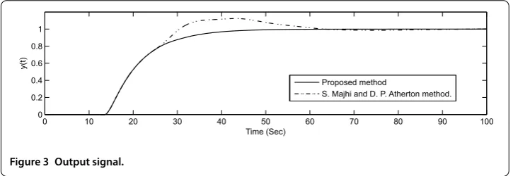
A comparison with the MoSP [] is made. First, is to note that the nominal delay used in the MoSP is lowerhˆnom = seconds in comparison with the initial nominal model used in our approachhˆnom = seconds, this was necessary, because if we use a delay ofhˆnom = seconds in the MoSP, this becomes unstable.
Figure clearly shows that the scheme is able to tackle the uncertainty in the delay, which leads to remarkable performance. Also, results demonstrate that the proposed scheme has a robust behaviour for uncertainties in modelling parameters of the plant.
Figure shows the value that takes the nominal delayHˆnom
k for the control law at each time interval, this is initialized in seconds,Hˆknom= . at seconds, which is a con-vergence time quite small, and taking into account the length of the real delay. Thus, good delay identification and good performance are achieved with a step as reference signal.
It can be seen that good results are obtained, despite the number of models (Nm= ) is small, and that theγijvalue is quite large, that is, . in comparison with requirements of Theorem .
Figure 4 Delay evolution through time.
Figure 5 Output signal for channel 1.
5.2 MIMO case
A complete knowledge of the delay-free part of the plant is assumed. The rational com-ponent of the considered plant is given by
Gdf(s) =
s–
. s+ . s+.
. s–.,
, ()
the matrix associated with the real delay of the plant is
H(s) =
e–.s e–.s e–.s e–.s
, ()
γij= ., k= [, , , , , , ], Tres= . seconds and the controllers are given by
C=
s+ s(s+)
s(s+)s+
, K=
, K=
. .
. ()
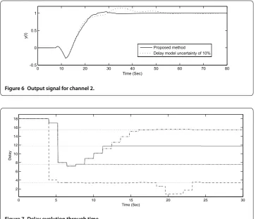
The system’s outputs are shown in Figures and for the channels and , respectively. The outputs are compared with a scheme having the model delay error of %. It can be seen that good results were obtained, since a fixed delay upper to % makes the system become unstable, although it is not shown in Figure . Notice that a finite value forγijand
Figure 6 Output signal for channel 2.
Figure 7 Delay evolution through time.
The nominal delay matrix at seconds is
ˆ Hknom=
e–.s e–.s e–.s e–.s
, ()
which is the same as (), the evolution of the delay through time is shown in Figure . As can be noticed, the convergence time is small in comparison with the channel delays, which permits the system’s stability.
5.3 Integrative case
In this section, the proposed approach is used over an integrative MIMO irrigation chan-nel model. The delay-free matrix of the irrigation chanchan-nel is given by
Gdf(s) =
⎡ ⎢ ⎣
. s
–.
s
. s
–. s .s
⎤ ⎥
⎦, ()
A modelling error of % is taking into account to show the robustness of the proposed approach
ˆ Gdf(s) =
⎡ ⎢ ⎣
. s
–.
s
.s –.s .s
⎤ ⎥
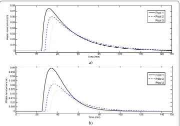
Figure 8 Water level for pool 1, 2 and 3. (a)PI control.(b)Proposed scheme.
and the actual delay is given by
H(s) =diag(., ., .), ()
Cis given by
C=
⎡ ⎢ ⎣
. s(s+)
s
. s(s+) s(s+).
⎤ ⎥
⎦, ()
andK=diag(, , ) andK=diag(., ., .). The way of selecting these values forK andKcontrollers is explained in detail in [].
The initial parameters used in the algorithm are given by:Tres= . seconds,Hˆknom=
diag(, , ) seconds, andk= [, , , , , , , , , , ]. Note that the number of models is lowNm= .
Figure shows the simulated water-level errors flows over upstream gates for the three pools, in response to a large step change in the flow out of pool . Figure (a) shows the simulation concerning a PI controller based on [] (where the used compensators are the same that the compensators used in the proposed scheme), where the model delay is con-stant,Hˆnom
k =diag(., ., .) (which correspond to a model delay error of±%). Figure (b) shows the output obtained with the proposed scheme, where the delay model is unknown.
Figure 9 Delay values for pools 1, 2 and 3.
scheme adjusts the controller through time, while in the other case, the control strategy is always fixed, this comparison is useful to show the effectiveness of the proposed scheme. Figure shows the delay evolution for the three pools, the obtained delay matrix is ˆ
Hk→∞=diag(., ., .). It is noteworthy that the identification is very precise, despite
the input signal is a step. Notice that the convergence time is fast, since in . minutes, all the delays are identified.
5.4 Time-varying delay
In this case, the pure delay term is given by
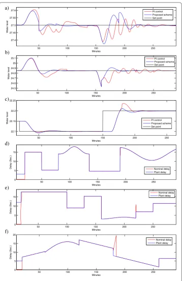
H(t) =diagh(t),h(t),h(t), () these are time-varying delays, whose variations are shown in Figure (d), (e) and (f ). As it can be seen, the delay varies arbitrarily, this is, in order to verify the optimal performance of the algorithm. The following scenario was simulated. At time minutes, all water levels were . m, . m and . m for pool , and , respectively. At time minutes the setpoint for the water level in pool was reduced from . m to . m, and at time minutes was augmented from . m to . m.
Figure (a), (b) and (c) shows the water level for pool , and , respectively. The pro-posed scheme is compared with PI controller propro-posed in [], where the delays are fixed in
ˆ
H=diag(., ., .). As expected, the simulation shows that in all three pools, better performance is achieved by the proposed scheme for time-varying delays.
Figures (d), (e) and (f ) shows the delay evolution for pools , and , respectively. It is noteworthy that the identification is very precise, and the presented Algorithm is able to follow the time-evolution of the delays. It can be seen that the approach can identify both abrupt as continuous changes in the delay.
6 Conclusion
Figure 10 Water level and delay identification.Pool 1.(a),(d). Pool 2.(b),(e). Pool 3.(c),(f).
been implemented online, using a multiple-model scheme, which is also a novel imple-mentation of pattern search methods.
simplification of the technical requirements on the input signal for the convergence results is an open question of research.
Finally, it is shown that the proposed approach is robustly stable, even when the ra-tional component of the system has a % error, which provides versatility and could be implemented in real systems. Moreover, simulation results showed that the identification is given with a great precision. Additionally, simulation results were presented for a time-varying delay case, where it is corroborated that the expected good results in practical sit-uations require readjustment of the model time delays. In authors’ opinion, pattern search methods constitute a powerful optimization technique for control-oriented applications such that it can be extended in future to the case, where the delay is time varying or for combined parametric and delay identification.
Competing interests
The authors declare that they have no competing interests.
Authors’ contributions
All authors contributed equally. All authors read and approved the final manuscript.
Author details
1Automatic and Electronic research group, Facultad de Ingeniería, Instituto Tecnológico Metropolitano (ITM), Medellín,
Antioquia, Colombia.2Departament de Telecomunicació i d’Enginyeria de Sistemes, Escola d’Enginyeria, Universitat Autònoma de Barcelona, Bellaterra, Barcelona, 08193, Spain. 3Institute of Research and Development of Processes, Facultad de Ciencia y Tecnología, Universidad del País Vasco, Vizcaya, P.O. 644, Bilbao, 48080, Spain.4Departamento de Electricidad y Electrónica, Facultad de Ciencia y Tecnología, Universidad del País Vasco, Vizcaya, P.O. 644, Bilbao, 48080, Spain.
Acknowledgements
This work was partially supported by the Spanish Ministry of Economy and Competitiveness through grant
DPI2012-30651, by the Basque Government (Gobierno Vasco) through grant IE378-10 and by the University of the Basque Country through grant UFI 11/07.
Received: 27 June 2013 Accepted: 25 September 2013 Published:19 Nov 2013
References
1. Dong, Y, Wei, J: Output feedback stabilization of nonlinear discrete-time systems with time-delay. Adv. Differ. Equ.
2012(73), 1-11 (2012)
2. Wei, F, Cai, Y: Existence, uniqueness and stability of the solution to neutral stochastic functional differential equations with infinite delay under non-Lipschitz conditions. Adv. Differ. Equ.2013(51), 1-12 (2013)
3. Alcántara, S, Pedret, C, Vilanova, R, Zhang, WD: Simple analytical min-max model matching approach to robust proportional-integrative-derivative tuning with smooth set-point response. Ind. Eng. Chem. Res.49(2), 690-700 (2010)
4. Lee, Y, Lee, J, Park, S: PID controller tuning for integrating and unstable processes with time delay. Chem. Eng. Sci.55, 3481-3493 (2000)
5. Ntogramatzidis, L, Ferrante, A: Exact tuning of PID controllers in control feedback design. IET Control Theory Appl.
5(4), 565-578 (2011)
6. Shi, D, Wang, J, Ma, L: Design of balanced proportional-integral-derivative controllers based on bilevel optimisation. IET Control Theory Appl.5(1), 84-92 (2011)
7. Zhang, WD, Sun, YX: Modified Smith predictor for controlling integrator/time delay processes. Ind. Eng. Chem. Res.
35, 2769-2772 (1996)
8. Majhi, S, Atherton, DP: Modified Smith predictor and controller for processes with time delay. Control Theory Appl.
146, 359-366 (1999)
9. Meng, D, Jia, Y, Du, J, Yu, F: Learning control for time-delay systems with iteration-varying uncertainty: a Smith predictor-based approach. IET Control Theory Appl.4(12), 2707-2718 (2011)
10. Normey-Rico, JE, Camacho, EF: Control of Dead-Time Processes. Springer, Berlin (2007)
11. De Paor, AM: A modified Smith predictor and controller for unstable processes with time delay. Int. J. Control41(4), 1025-1036 (1985)
12. Herrera, J, Ibeas, A, Alcantara, S, de la Sen, M: Multimodel-based techniques for the identification and adaptive control of delayed multi-input multi-output systems. IET Control Theory Appl.5(1), 188-202 (2011)
13. Garcia, CA, Ibeas, A, Herrera, J, Vilanova, R: Inventory control for the supply chain: an adaptive control approach based on the identification of the lead-time. Omega40, 314-327 (2012)
14. Herrera, J, Ibeas, A, Alcantara, S, Vilanova, R: Multimodel-based techniques for the identification of the delay in mimo systems. In: Proceedings of the 2010 American Control Conference, Marriott Waterfront, Baltimore, MD, USA, June 30-July 02 (2010)
16. Torczon, V: On the convergence of pattern search algorithms. SIAM J. Optim.7(1), 1-25 (1997)
17. Pan, I, Das, S, Gupta, A: Tuning of an optimal fuzzy PID controller with stochastic algorithms for networked control systems with random time delay. ISA Trans.50, 21-27 (2011)
18. Dong, Y, Liu, J: Exponential stabilization of uncertain nonlinear time-delay systems. Adv. Differ. Equ.2012(180), 1-15 (2012)
19. Gouaisbaut, F, Dambrine, M, Richard, JP: Robust control of delay systems: a sliding mode control design via LMI. Syst. Control Lett.46, 219-230 (2002)
20. Sangapate, P: New sufficient conditions for the asymptotic stability of discrete time-delay systems. Adv. Differ. Equ.
2012(28), 1-8 (2012)
21. Xiang, M, Xiang, Z: Reliable control of positive switched systems with time-varying delays. Adv. Differ. Equ.2013(25), 1-15 (2013)
22. Liu, T, Gao, F: Closed-loop step response identification of integrating and unstable processes. Chem. Eng. Sci. (2010). doi:10.1016/j.ces.2010.01.013
23. Bogani, C, Gasparo, MG, Papini, A: Generalized pattern search methods for a class of nonsmooth optimization problems with structure. J. Comput. Appl. Math.229, 283-293 (2009)
24. Liu, L, Zhang, X: Generalized pattern search methods for linearly equality constrained optimization problems. Appl. Math. Comput.181, 527-535 (2006)
25. Jelali, M: Estimation of valve stiction in control loops using separable least-squares and global search algorithms. J. Process Control18, 632-642 (2008)
26. Negenborn, RR, Leirens, S, De Schutter, B, Hellendoorn, J: Supervisory non linear MPC for emergency voltage control using pattern search. Control Eng. Pract.17, 841-848 (2009)
27. Ibeas, A, de la Sen, M: Artificial intelligence and graph theory tools for describing switched linear control systems. Appl. Artif. Intell.20(9), 703-741 (2006)
28. Bernstein, DS: Matrix Mathematics. Princeton University Press, Princeton (2005)
29. Marchetti, G, Scali, C, Lewin, DR: Identification and control of open-loop unstable processes by relay methods. Automatica37, 2049-2055 (2001)
30. Audet, C, Dennis, JE: Mesh adaptive direct search algorithms for constrained optimization. SIAM J. Optim.17, 188-217 (2006)
10.1186/1687-1847-2013-331