Simulation and Experiment for Induction Motor Control Strategies

(1)

University of Windsor University of Windsor

Scholarship at UWindsor

Electronic Theses and Dissertations Theses, Dissertations, and Major Papers

2011

Simulation and Experiment for Induction Motor Control Strategies

Zhi Shang

University of Windsor

Follow this and additional works at: https://scholar.uwindsor.ca/etd

Recommended Citation Recommended Citation

Shang, Zhi, "Simulation and Experiment for Induction Motor Control Strategies" (2011). Electronic Theses and Dissertations. 5387.

https://scholar.uwindsor.ca/etd/5387

This online database contains the full-text of PhD dissertations and Masters’ theses of University of Windsor students from 1954 forward. These documents are made available for personal study and research purposes only, in accordance with the Canadian Copyright Act and the Creative Commons license—CC BY-NC-ND (Attribution, Non-Commercial, No Derivative Works). Under this license, works must always be attributed to the copyright holder (original author), cannot be used for any commercial purposes, and may not be altered. Any other use would require the permission of the copyright holder. Students may inquire about withdrawing their dissertation and/or thesis from this database. For additional inquiries, please contact the repository administrator via email

(2)

Simulation and Experiment for Induction Motor Control

Strategies

by

Zhi SHANG

A Thesis

Submitted to the Faculty of Graduate Studies

through Mechanical Engineering

in Partial Fulfillment of the Requirements for

the Degree of Master of Applied Science at the

University of Windsor

Windsor, Ontario, Canada

2011

(3)

Simulation and Experiment for Induction Motor Control

Strategies

by

Zhi SHANG

APPROVED BY:

Dr. J. Johrendt, Department Reader

Department of Mechanical, Automotive & Material Engineering

Dr. H. Wu, Outside Department Reader

Department of Electrical and Computer Engineering

Dr. B. Zhou, Advisor

Department of Mechanical, Automotive & Material Engineering

Dr. C. Novak, Chair of Defense

(4)

AUTHOR’S DECLARATION OF ORIGINALITY

I hereby certify that I am the sole author of this thesis and that no part of this

thesis has been published or submitted for publication.

I certify that, to the best of my knowledge, my thesis does not infringe upon

anyone’s copyright nor violate any proprietary rights and that any ideas, techniques,

quotations, or any other material from the work of other people included in my thesis,

published or otherwise, are fully acknowledged in accordance with the standard

referencing practices. Furthermore, to the extent that I have included copyrighted

material that surpasses the bounds of fair dealing within the meaning of the Canada

Copyright Act, I certify that I have obtained a written permission from the copyright

owner(s) to include such material(s) in my thesis and have included copies of such

copyright clearances to my appendix.

I declare that this is a true copy of my thesis, including any final revisions, as

approved by my thesis committee and the Graduate Studies office, and that this thesis

(5)

ABSTRACT

The Induction motor has been widely used in industry and is considered as

the best candidate for electrical vehicle (EV) applications due to its advantages such

as: simple design, ruggedness, and easy maintenance. However, the precise control of

induction motor is not easy to achieve, because it is a complicated nonlinear system,

the electric rotor variables are not measurable directly, and the physical parameters

could change in different operating conditions. So the control of an induction motor

becomes a critical issue, especially for the EV applications in which both fast

transient responses and excellent steady state speed performance are required.

Three induction motor control algorithms (field orientation control,

conventional direct torque control, and stator flux orientated sensorless direct torque

control) are introduced in this thesis and a specific comparison is given among three

of them. The main focus of this work is to design an induction motor control system

using the three algorithms mentioned above, to analyze the performances of different

control methods, and to validate these algorithms experimentally, comparing the

(6)

DEDICATION

(7)

ACKNOWLEDGEMENTS

I wish to express my sincere gratitude to my supervisor Dr. B. Zhou, who has

been a constant source of guidance, support and encouragement throughout my

graduate studies. His extensive knowledge, rigorous research attitude, diligent

working and creative thinking have inspired me and will definitely benefit my future

career.

My gratitude should also be given to Dr. J. Johrendt and Dr. H. Wu for

serving as my committee members, giving me valuable suggestions and taking the

time to revise my thesis. I would like to dedicate all my thanks to them.

The experimental part of this project was the most challenging part. I could

not have done this without the help from the technicians in Mechanical Engineering

Department: Mr. Andy Jenner and Mr. Patrick Seguin, also the technician in Electrical

Engineering Department: Mr. Frank Cicchello. I would like to thank them with

enormous appreciation for their help and advice.

I also would like to express my thanks to Mr. Ahmad Fadel, Mr. Rui Hu, and

Mr. Esmaeil Navaei Alvar. It has been a great pleasure studying and working with

them. The discussions, comments and suggestions they gave to me allowed me to

improve my research in many aspects.

Finally I would like to thank my parents for their love, support and sacrifices.

(8)

LIST OF FIGURES

Figure 1: Ideal performance characteristics for a vehicle traction power plant ... 2

Figure 2: Typical characteristics of a gasoline engine ... 2

Figure 3: A multi-gear transmission vehicle gear ratio vs. speed ... 3

Figure 4: Typical characteristics of an electric motor ... 4

Figure 5: Classification of electric motor ... 4

Figure 6: Permanent magnet synchronous motors ... 5

Figure 7: Switched reluctance motors ... 6

Figure 8: Induction motors ... 6

Figure 9: Squirrel cage induction motor cross section ... 15

Figure 10: Current space vectors ... 16

Figure 11: Clarke transformation of three-phase currents ... 17

Figure 12: Park transformation of two-phase currents... 18

Figure 13: Alpha component of the induction motor equivalent-circuit ... 19

Figure 14: Beta component of the induction motor equivalent-circuit ... 19

Figure 15: PWM techniques for time invariant signals ... 24

Figure 16: PWM techniques for time variant signals ... 24

Figure 17: Three-phase voltage source inverter ... 25

Figure 18: Voltage source inverter output vectors in the Alfa-beta plane ... 26

Figure 19: Phase voltage of SVPWM ... 27

Figure 20: Line to line voltage of SVPWM ... 27

Figure 21: The transfer function G(p) ... 30

Figure 22: The electromagnetic torque is directly controlled by two decoupled currents 30 Figure 23: The rotating angle between the stationary and rotational frames ... 31

Figure 24: The calculation of flux magnitude and angle ... 32

Figure 25: DFOC system diagram ... 32

Figure 26: The system diagram of IFOC ... 34

Figure 27: Three phase stator currents in FOC ... 35

Figure 28: Two phase currents after Clarke transformation in FOC ... 35

Figure 29: Torque response based on the requirement ... 36

Figure 30: Decoupled current Iqs which is responsible for generating torque ... 36

Figure 31: Rotor flux trajectory in FOC ... 36

Figure 32: Decoupled current Ids which is responsible for generating flux ... 37

Figure 33: Equivalent- circuit of induction motor in the stationary frame ... 38

Figure 34: Stator flux and Rotor flux in stationary frame ... 39

Figure 35: Eight possible voltage vectors formed by a voltage source inverter ... 39

Figure 36: The corresponding stator flux changes ... 40

Figure 37: The two-level hysteresis controller for stator flux... 41

Figure 38: Stator flux trajectory ... 42

Figure 39: The three-level hysteresis-controller for electromagnetic torque ... 42

Figure 40: Block diagram of Conventional DTC ... 43

(11)

Figure 42: Block diagram of SFO-Sensorless DTC ... 47

Figure 43: Three phase stator currents in conventional DTC ... 47

Figure 44: Two phase currents after Clarke transformation in conventional DTC ... 48

Figure 45: Torque response with command in conventional DTC ... 48

Figure 46: Circular stator flux trajectory in conventional DTC ... 49

Figure 47: Speed command vs. time in Scenario 1 ... 51

Figure 48: Torque command vs. time in Scenario 1 ... 51

Figure 49: Speed response of FOC in Scenario 1 ... 52

Figure 50: Speed response of conventional DTC in Scenario 1 ... 52

Figure 51: Speed response of SFO-Sensorless DTC in Scenario 1 ... 53

Figure 52: Torque response of FOC in Scenario 1 ... 54

Figure 53: Torque response of conventional DTC in Scenario 1 ... 54

Figure 54: Torque response of SFO-Sensorless DTC in Scenario 1 ... 54

Figure 55: Currents response of FOC in Scenario 1 ... 55

Figure 56: Currents response of conventional DTC in Scenario 1 ... 55

Figure 57: Currents response of SFO-Sensorless DTC in Scenario 1 ... 56

Figure 58: Speed command vs. time in Scenario 2 ... 57

Figure 59: Torque command vs. time in Scenario 2 ... 57

Figure 60: Speed response of FOC in Scenario 2 ... 58

Figure 61: Speed response of conventional DTC in Scenario 2 ... 58

Figure 62: Speed response of SFO-Sensorless DTC in Scenario 2 ... 58

Figure 63: Torque response of FOC in Scenario 2 ... 59

Figure 64: Torque response of conventional DTC in Scenario 2 ... 59

Figure 65: Torque response of SFO-Sensorless DTC in Scenario 2 ... 59

Figure 66: Currents response of FOC in Scenario 2 ... 60

Figure 67: Currents response of conventional DTC in Scenario 2 ... 60

Figure 68: Currents response of SFO-Sensorless DTC in Scenario 2 ... 61

Figure 69: Hardware schematic diagram of induction motor control system ... 62

Figure 70: Experimental three phase stator currents in FOC ... 65

Figure 71: Experimental two phase currents in FOC ... 65

Figure 72: Experimental decoupled current Ids vs. time ... 66

Figure 73: Experimental decoupled current Iqs vs. time ... 66

Figure 74: Experimental SVPWM phase voltage waveform ... 67

Figure 75: Experimental torque response for DTC ... 68

Figure 76: Experimental stator flux trajectory in DTC ... 68

Figure 77: Decoupled current Ids in experiment ... 69

Figure 78: Decoupled current Ids in simulation ... 69

Figure 79: Decoupled current Iqs in experiment ... 70

Figure 80: Decoupled current Iqs in simulation ... 70

Figure 81: DTC stator flux trajectory in experiment ... 71

Figure 82: DTC stator flux trajectory in simulation ... 71

Figure 83: DTC torque response in experiment ... 72

(12)

LIST OF SYMBOLS

α Axis of stationary frame

β Axis of stationary frame

d Axis of rotating frame

q Axis of rotating frame

n Synchronous speed in revolutions per minute

f Frequency of the power source

P The number of poles

n Slip speed

n Mechanical shaft speed of the motor

s Slip ratio

i Stator current

i Rotor current

i , , Three phase current

Ψ Stator flux

Ψ Rotor flux

Ψ Mutual flux

i Stator current component in Alfa-axis

i Stator current component in Beta-axis

i Rotor current component in Alfa-axis

i Rotor current component in Beta-axis

i Stator current component in d-axis

i Stator current component in q-axis

i Rotor current component in d-axis

i Rotor current component in q-axis

R Resistance

(13)

R

u

Rotor resistance

Stator voltage

u Stator voltage component in Alfa-axis

u Stator voltage component in Beta-axis

p Differential operator d/dt

L Stator inductance

L Rotor inductance

L Mutual inductance

l Inductance

ω Rotor mechanical angular velocity

ω Synchronous angular velocity

ω Slip angular velocity

θ Synchronous angle

θ Rotor flux angle in synchronous frame

θ Phase angle of voltage vector um

θ Stator flux angle

θ Angle between rotor flux and stator flux

T Electromagnetic torque

TL Load torque

B Stator magnetic flux density

B Rotor magnetic flux density

K ~K Torque constant

J Rotor’s moment of inertia

V DC main bus Voltage

V _, _, Phase voltage

V _{, ,} Line to line voltage

S , , Switching variable vectors

V ~V Space voltage vectors

(14)

S Flux flag

∆E Flux error

Ψ Flux hysteresis controller boundary

S_T Torque flag

∆E_T Torque error

T Torque hysteresis controller boundary

S K Sector number, K=1~6

, ref Reference values

(15)

CHAPTER I. INTRODUCTION

1.1 Background

The development of internal combustion engine vehicles is one of the greatest

achievements in the automotive industry for the past a few centuries. Automobiles

have made great contributions to the growth of modern technology, economy, even

cultures by satisfying many of the needs for mobility in our daily life.

However, the large numbers of automobiles which are being used all around the world

have caused serious problems for the environment and human life. Air pollution,

global warming, and the rapid depletion of the earth’s petroleum resources are now

problems of primary concern. The environmental issues and oil crisis compel people to develop clean, efficient vehicles solutions for urban transportation.

In the past a few decades, lots of research and development activities related to the

automotive industry started emphasizing the development of clean, low/zero emission,

and high efficiency transportation. So electric vehicles (EVs), hybrid electric vehicles

(HEVs), and fuel cell vehicles became popular again and have been typically

proposed to replace conventional vehicles in the near future. The electric vehicle is

the first consideration for its zero emissions feature [1, 2].

1.2 Power Plant Characteristics

For vehicular applications, the ideal performance characteristic of a power plant is a

constant power output over the full speed range. Consequently, the torque varies with

speed hyperbolically as shown in Figure 1 [2, 3]. With this ideal profile, the maximum

power of the power plant will be available at any vehicle speed, therefore yielding the

(16)

Figure 1: Ideal performance characteristics for a vehicle traction power plant

The most commonly used power plants for vehicles are no doubt the internal

combustion engine. The typical characteristics of an internal combustion engine are

shown in Figure 2[2]. Obviously, it is far from the ideal torque–speed profile curve.

At the idle speed region, it operates in a smooth condition, but the maximum torque is

achieved at an intermediate speed. With the speed further increasing, the torque

decreases.

Instead of occurring at the very beginning, the maximum power happens at a high

speed. Beyond this speed, the engine power decreases. Furthermore, the internal

combustion engine has a relatively flat torque–speed profile, as compared with an

ideal power plant shown in Figure 2. Therefore, a multi-gear transmission is

commonly employed to modify the torque-speed profile, as shown in Figure 3 [2].

(17)

Figure 3: A multi-gear transmission vehicle gear ratio vs. speed [2]

The electric motor is another candidate as a vehicle power plant, and becoming more

and more important with the rapid development of electric and hybrid electric

vehicles.

Motors are the work horses of electric vehicles drive systems. An electric motor

converts electrical energy from the energy storage unit to mechanical energy that

drives the wheels of the vehicle. In the traditional vehicle case, the engine must ramp

up before full torque can be provided [2]; however, in the case of electric motor, the

full torque could be provided at low speed ranges [3]. This characteristic is very

important; it gives the vehicle an excellent acceleration at the beginning. Also, other

important characteristics of the motor include good control abilities, fault tolerance

abilities, and high efficiency [4].

The speed–torque characteristics of electric motors are much closer to the ideal one,

as shown in Figure 4 [2]. The speed starts from zero and generally increases to its

base value. During this process, the voltage increases to its rated value as well, and

the flux remains constant [3]. A constant torque is generated in this speed range from

zero to base speed. Beyond the base speed, the voltage remains as a constant and the

output power will also remain as a constant. Thus, the output torque declines

(18)

motor is close to the ideal one, people only need to use a single-gear or double-gear

transmission to modify the vehicle performance to receive their desired design

requirements [2].

Figure 4: Typical characteristics of an electric motor [2]

1.3 Electric Motor

The motor drives for EVs can be classified into two groups, as shown in Figure 5:

y Commutator motors (also known as DC motors)

y Commutatorless motors (known as AC motors)

Figure 5: Classification of electric motor

1.3.1 Permanent Magnet Synchronous Motor (PMSM)

Instead of using the windings for the rotor, the PMSM’s rotor is made of magnetic

(19)

motor. The magnetic flux in a PMSM is generated from the magnetic materials on

rotor. And absence of rotor windings gives PMSMs some advantages such as high

efficiency and higher power density [5].

On the other side, the absence of field windings makes the flux weakening capability

of PMSM’s constrained, and eventually limits their speed ranges in the constant

power region [6]. Also, the permanent magnet is very sensitive to the temperature, this

will certainly lead to a demagnetization problem, and sometimes a special cooling

system is necessary for a PMSM drive system.

Figure 6: Permanent magnet synchronous motors [7]

1.3.2 Switched Reluctance Motor

The switched reluctance motor is an electric motor which runs by reluctance torques

[8]. It is another potential candidate due to some important features such as rugged

structure, high power density, and insensitivity to high temperatures [9].

The wound field coils are fixed on the stator, but the rotor has no magnets or coils

attached. When the opposite poles of the stator get energized, the rotor will become

aligned. In order to achieve a full rotation of the motor, the windings must be

energised in the right sequence [8].

(20)

noise, and instabilities caused by the energising sequence [9-11].

Figure 7: Switched reluctance motors [12]

1.3.3 Induction Motor

The induction motor is a type of AC motor; it is called an induction motor because the

working principles are based on electromagnetic induction. The energy is transformed

through the rotating magnetic fields in induction motor. The three-phase currents in

the stator side create an electromagnetic field which interacts with the electromagnetic

field in the rotor bars, and then the resultant torque will be produced by the Lorentz’

law. Therefore, the electrical energy could be transformed into mechanical energy.

Induction motors are the preferred choice for industrial applications due to their

rugged structure, low price and easy maintenance [13].

(21)

1.3.4 Comparison of Three AC Motors

Table 1: Comparison among three AC motors [5-11]

Item Induction Motor PM Motor SR Motor

Power density Medium High Higher

Overload capacity (%) 300-500 300 300-500

Peak efficiency (%) 94-95 95-97 90

Load efficiency (%) 90-92 85-97 78-86

Range of speeds (r/min) 12K-20K 4K-10K More than 15K

Reliability Good Better Good

Volume Medium Small Small

Mass Medium Light Light

Control Performance Good Good Good

Manufacturing costs Medium High Medium

The PMSM is a popular candidate because of its high power density, high efficiency

and compact volume. But the disadvantage is the magnetic materials used in the

PMSM are really expensive, and they need to be well maintained for the reason of

magnet corrosion or demagnetization. The SRM is another promising candidate for

EV applications, because of its simple structure, fault tolerant operation, and wide

speed range at constant power. However, the disadvantages of the SRM are its high

torque ripples and low efficiency [11, 15]. As a result of these researches, the

induction motor is considered as the best candidate for the most of EVs applications

[3, 5]. Intelligent, reliable and commercialized control systems of AC induction

motors are being developed based on power electronic devices and digital signal

(22)

1.4 Research Objectives and Thesis Outline

Since an induction motor is a complicated nonlinear system, the electric rotor

variables are not measurable directly, and the physical parameters of an induction

motor are often imprecisely known. Meanwhile, the induction motor used in electric

vehicle applications usually requires both fast transient responses and excellent steady

state speed performance. All of these make the control of induction a challenging

problem.

Lots of research has been done in the area of controlling an induction motor, some

control methods result in an excellent steady state performance (e.g. Field Orientation

Control (FOC)), others provide a great dynamic response (e.g. Direct Torque Control

(DTC)), and there are some algorithms aiming at coupling the advantages from both

side (e.g. stator flux orientated sensorless DTC). But no one has given a specific

comparison among three of them. Thus an elaborate comparison is very necessary.

The main focus of this work is to design an induction motor control system using

three algorithms mentioned above: FOC, DTC, and stator flux orientated sensorless

DTC. The performances of different control algorithms will be analyzed, at the same

time, these algorithms will be validated experimentally. Finally, the simulation results

will be compared with experimental ones.

Thus, the scope of work of this project can be outlined by the following steps:

Step 1. Develop simulation models for each control algorithm.

Step 2. Compare simulation results for each control algorithm.

Step 3. Size the components for an induction motor control test bench and design

peripheral circuits.

Step 4. Validate the effectiveness of the controller experimentally

(23)

This thesis is organized as follows:

The literature review for this work is summarized in Chapter 2. Chapter 3 presents the

induction motor modeling basics, including the modeling tools and the modeling

equations. The theory and implementation of filed orientation control for an induction

motor will be introduced in Chapter 4, and in Chapter 5, the Direct Torque Control

and Stator flux oriented sensorless DTC will be presented. Chapter 6 will focuses on

the simulation results analysis, and in Chapter 7, the hardware setup and experimental

results will be presented. The overall conclusions and future work are presented in

(24)

CHAPTER II. LITERATURE REVIEW

2.1 Induction Motor Control Algorithms

The most commonly used control methods for AC induction motors are field

orientation control, and direct torque control.

2.1.1 Field Oriented Control

The vector control techniques started developing around 1970 [16]. A few types of

vector control, such as rotor flux oriented, stator flux oriented and mutual flux

oriented are published one after another. No matter what kind of vector control, they

are all subjected to imitate a separately excited DC motor, in which the

electromagnetic torque and magnetic field can be controlled separately.

Field oriented control (FOC) has the capability of controlling both the field-producing

and the torque-producing currents in a decoupled way [16]. For different applications,

people might choose different flux orientation for some special demands. However,

only the rotor flux oriented control achieves a complete decoupled system.

The field oriented control refers in particular to the rotor flux oriented type of vector

control. Furthermore, the field oriented control can be classified into indirect or direct

field oriented control, depending on how to obtain the rotor flux orientation.

The direct FOC obtains the orientation of the mutual flux by installing a hall-effect

sensor inside the induction motor. However, using these type sensors is expensive and

inconvenient, because special modifications need to be made in order to place the flux

sensors. Furthermore, it is impossible to sense the rotor flux, so we have to sense the

mutual flux directly and then calculate out the rotor flux information.

(25)

By using the signals from the motor terminals such as three phase currents and rotor

rotating speed, the rotor flux orientation can be estimated using motor state equations.

Indirect FOC does not have the problems that direct FOC does, which makes it

popular in most applications.

2.1.2 Direct Torque Control

Direct torque control (DTC) was introduced in Japan by Takahashi and Nagochi [17]

and also in Germany by Depenbrock [18]. This control algorithm does not follow the

well developed DC motor control strategies. Instead of doing the coordinate

transformations to decouple the electromagnetic torque and magnetic field, it employs

a bang-bang control by using the hysteresis-controller. The bang-bang control works

perfectly with the semiconductor inverter. As the name indicates, the most important

feature of direct torque control is that it controls the electromagnetic torque and stator

flux directly.

The typical DTC includes two hysteresis controllers [19]. Usually before

implementing the hysteresis-controller, the actual stator flux is calculated from the

stator voltages, and electromagnetic torque is calculated from the stator voltages and

stator currents.

Therefore, the DTC control method strongly depends on the stator variables. As the

stator voltage changes, the stator flux follows rapidly while the rotor flux changes

slowly. This will modify the angle between stator and rotor fluxes and consequently

the electromagnetic torque will be increased or decreased.

In the hysteresis-control section, a two-level stator flux hysteresis controller and a

three-level torque hysteresis controller are commonly employed in the DTC scheme.

One of the two flags will be generated from the stator flux hysteresis controller, when

(26)

flags will come out from the torque hysteresis controller. Furthermore, a sector

number in which the stator flux vector lies need to be calculated out.

Using flux flag, torque flag, and flux sector number together as inputs, a voltage

lookup table is then employed here. The appropriate voltage vector for the inverter is

selected from the lookup table based on whether a need to increase or decrease the

torque and stator flux. DTC attracts many researchers because of its fast torque

response and simple control method [19, 20].

2.2 Comparison of Induction Motor Control Algorithms

An objective comparison between FOC and DTC is actually difficult to make since

each author has his/her own specific demands and predilections. The most distinct

differences can be given as: the orientation of FOC is usually on rotor flux while that

of DTC is always on stator flux. Another difference is that two current controllers are

necessary for FOC but which are replaced by a switching table in DTC.

The presence of a current controller could be an advantage of regulating the currents

fluctuations. In practical operations, however, it is a limiting factor in terms of the

transient performance. On the other hand, the two separate hysteresis controllers for

flux and torque in DTC are able to immediately apply the maximum voltage to the

motor which results in a better torque response.

Generally speaking, DTC provides a better dynamic torque response while FOC

provides a better steady state behavior. But for vehicular applications, both steady

state and dynamic performance are important to the system.

So it is obvious to imagine that if there is a control method which combines the

advantages of FOC and DTC together, then both steady state and dynamic

(27)

combining FOC and DTC to improve both the steady state as well as dynamic

performance, [21-25].

One of the developed methods is stator flux orientated sensorless direct torque control.

This control method is based on direct torque control, so the torque and flux responses

can be guaranteed. At the same time the stator flux orientation technique is applied to

predict the rotor speed. The flux orientation is a necessary part in FOC and because of

this FOC achieves the decoupled currents and shows an excellent speed behavior.

Thus, a DTC scheme with the flux orientation technique will surely provide a well

regulated speed performance. In addition, the speed sensor can be eliminated from the

system, since the rotor speed can be estimated instead of being measured. The

absence of the speed sensor, either optical encoder or hall-effect speed sensor will

(28)

CHAPTER III. INDUCTION MOTOR MODELING

3.1 Induction Motor Basics

Three phase induction motors are rugged, cheap to produce and easy to maintain.

They can run at a nearly constant speed from zero to full load. The design of an

induction motor is relatively simple and consists of two main parts, a stationary stator

and a rotating rotor. There are two main classes of the induction motor differing in the

way their rotors are wound: the wound induction motor and the squirrel cage

induction motor.

The motor discussed in this thesis is a three phase squirrel cage induction motor. The

rotor of a squirrel cage induction motor consists of aluminum bars which are short

circuited by connecting them to two end rings so that rotor generates the induction

current and magnetic field by itself. This makes the AC induction motor a robust,

rugged and inexpensive candidate for motor drive systems [26].

The structure of a squirrel cage induction motor is shown in Figure 9. In an induction

motor, the alternating currents feed from three phase terminals and flow through the

stator windings, producing a rotating stator flux in the motor [26]. The rotating speed

of this magnetic field is defined as synchronous speed, and related to the number of

poles of the induction motor and the frequency of power source.

120 (3.1)

e

sync

f

n

rpm

P

=

where fe is the power source frequency, P is the number of poles and nsync is the

synchronous speed in revolutions per minute.

The rotating magnetic field from the stator will induce a voltage in the rotor bars,

since the rotor bars are short-circuited, a large circulating current will be generated in

(29)

field. Because of Lorentz’s law, a tangential electromagnetic force will be generated

on the rotor bars, and the sum of forces on each rotor bar produces a torque that

eventually drives the rotor in the direction of the rotating field.

Figure 9: Squirrel cage induction motor cross section [14]

When the rotating magnetic field is first generated, the rotor is still in its rest

condition. However, the rotor will accelerate rapidly in order to keep up with the

rotating stator flux. As the rotor speed increases, the rotor bars are not cut as much by

the rotating field, so the voltage in the rotor bars decreases. If the rotor speed equals to

the flux speed, the rotor bars will no longer be cut by the field and the rotor will start

to slow down [26]. This is why induction motors are also called asynchronous motors

because the rotor speed will never equal the synchronous speed. The difference

between the stator and rotor speed is defined as the slip speed:

(3.2)

slip sync m

n =n −n

where nslip is the slip speed

nsyncis the speed of the rotating magnetic field

nm is the mechanical shaft speed of the motor

Also, a slip ratio can be defined as:

(3.3)

sync m

sync

n n

s

n

− =

(30)

s = 0 (3.4)

if the rotor stops moving

s = 1 (3.5)

3.2 Space Vectors

By using space vectors in the induction motor modeling, all the complex state

variables can be efficiently defined [27]. Variables such as the three phase voltages,

currents and fluxes of induction motors can be analyzed and described easily and

conveniently.

The three phase axes are defined by the vectors:

e

j0o ,

e

j120oand

e

j240o . The stator windings and stator current space vector in the complex plane are shown in below.

Figure 10: Current space vectors

The space vector of the stator current

i

_s can be described by:

0 120 240

(3.6)

j j j

s as bs cs

i =i ⋅e o + ⋅i e o + ⋅i e o

where subscript s refers to the stator of the induction motor, a, b, and c are the three

phase axes.

Furthermore, the rotor current can be described by:

0 120 240

(3.7)

j j j

r ar br cr

(31)

where subscript r refers to the rotor of the induction motor.

3.3 The Coordinate Transformation of Space Vectors

The modeling, analysis and control design of induction can be significantly simplified

by using coordinate transformations. A three-phase variable can be transferred into a

two-phase variables [28]; also a stationary variable can be transferred into a rotational

one [29]. This transformation usually includes the following two steps:

y The Clarke transformation

y The Park transformation

3.3.1 Clarke Transformation

The Clarke transformation transfers a three-phase system into a two-phase system.

Take the currents, for example:

2 1 1

3 3 3

(3.8)

3 3

0

3 3

a

b

c

i i

i α

β

⎛ ₋ ₋ _{⎞ ⎛ ⎞}

⎜ ⎟

⎛ ⎞ ⎜ ⎟

⎜ ⎟

= ⋅

⎜ ⎟ ⎜ ⎟

⎜ ⎟ ⎜ _{⎟ ⎜ ⎟}

⎝ ⎠ _⎜ ₋

⎟ ⎝ ⎠

⎝ ⎠

Figure 11: Clarke transformation of three-phase currents

In this thesis,

( , , )

a b c

⇒

( , )

α β

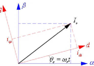
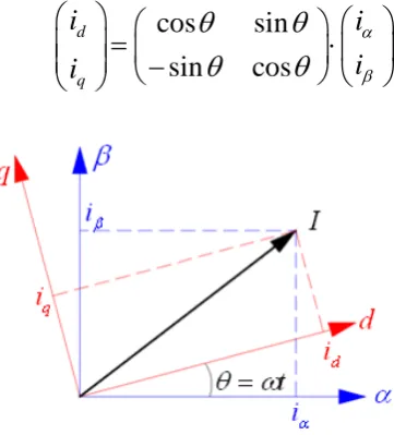
is used to represent the Clarke transformation.

3.3.2 Park Transformation

(32)

cos

sin

(3.9)

sin

cos

d

q

i

α

β

θ

⎛ ⎞

_⎛

_⎞

_{⎛ ⎞}

=

⋅

⎜ ⎟

_⎜

_⎟

_{⎜ ⎟}

⎜ ⎟

_⎝

₋

_{⎠ ⎝ ⎠}

⎝ ⎠

Figure 12: Park transformation of two-phase currents

Here

( , )

α β

⇒

( , )

d q

is used to represent the Park transformation.

3.4 Modeling Equations

The induction motor modeling usually contains three parts: flux equations, voltage

equations and torque equations [27].

3.4.1 Flux Equations

There are three kinds of fluxes: stator flux, rotor flux and mutual flux. The stator flux

and rotor flux vectors can be expressed in terms of stator current i_s and rotor current

r

i , given below:

(3.10)

s

L I

s s

L I

m r

Ψ =

+

(3.11)

r

L I

r r

L I

m s

Ψ =

+

whereL_sandL_rare the stator inductance and the rotor inductance, respectively; L_mis

the mutual inductance between the stator and rotor windings.

3.4.2 Voltage Equations

(33)

in different coordinate frames. Three kinds of coordinate frames are commonly used

to describe the induction motors [27]. They are:

y Stationary frame;

y Synchronous rotating frame;

y Field orientation synchronous frame.

3.4.2.1 Voltage Equations in Stationary Frame

The induction motor usually has three sets of stator windings, and the rotor can be

considered as three sets of windings as well [27]. Both stator and rotor can be

represented by inductance and resistance in an equivalent-circuit. Using the Clarke

transformation, the three-phase induction motor model can be expressed as an

equivalent two-phase model [27]. The equivalent circuits in the stationary frame of

the induction motor are shown in Figure 13 and 14:

Figure 13: Alpha component of the induction motor equivalent-circuit

Figure 14: Beta component of the induction motor equivalent-circuit

Based on the Kirchhoff’s voltage law (KVL), the stator and rotor voltage equations

can be expressed as:

(3.12)

s s s s

(34)

(3.13)

s s s s

u_β =i R_β + p

ψ

_β

0=i R_α_r _r + p

ψ

_α_r +

ω ψ

_r _β_r (3.14)

0=i Rβr r + p

ψ

βr −

ω ψ

r αr (3.15)

where ω ψ_r _β_rand ωψ_r _α_rare rotating velocity emf and p is the differential operator.

Substituting eq. 3.10 and 3.11 into eq. 3.12 and eq. 3.13, the stator voltage equations

can be rewritten:

(

)

(3.16)

s s s s m r

u

_α

=

R

+

L p i

_α

+

L pi

_α

( ) (3.17)

s s s s m r

u_β = R +L p i_β +L pi_β

Also, the rotor voltage equations can be rewritten as:

0= L pi_m _α_s +(R_r +i p i_r )_α_r +

ω

_rL i_m _β_s +

ω

_rL i_r _β_r (3.18)

0= L pi_m _β_s +(R_r +i p i_r )_β_r −

ω

_rL i_m _α_s −

ω

_rL i_r _α_r (3.19)

The relationship of voltages and currents can be given in matrix form from the four

voltage equations:

( ) 0 0

0 ( ) 0

(3.20) ( ) 0 ( ) 0 s

s s m

s

s s m

s

r

m r m r r r r

r

m r m r r r r

i

R L p L p

u

i

R L p L p

u

i

L p L R L p L

i

L L p L R L p

α α β β α β

ω

+ ⎛ ⎞ ⎛ ⎞ ⎛ ⎞ ⎜ ⎟ ⎜ ⎟ ⎜ ⎟ ₊ ⎜ ⎟ ⎜ ⎟ ⎜ _{⎟ =} _{⋅⎜ ⎟} ⎜ ⎟ ⎜ ⎟ + ⎜ ⎟ ⎜ ⎟ ⎜ ⎟ ₋ ₋ ₊ _⎜ _⎟ ⎝ ⎠ ⎝ ⎠ ⎝ ⎠

where ω_r is rotor speed.

3.4.2.2 Voltage Equations in Synchronous Rotating Frame

This is a rotary frame and the rotating speed isω_e. Using the Park transformation, eq.

3.12, and 3.13 can be expressed in the d-q synchronous rotating reference frame, so

the stator voltage equations can be rewritten as:

(3.21)

ds ds s ds e qs

(35)

(3.22)

qs qs s qs e ds

u =i R + p

ψ

+

ω ψ

The last terms in eq. 3.21 and eq. 3.22 can be defined as speed emf as they are directly

related with the synchronous speed of the motor. When ω_e=0, these equations turn

back to stationary forms.

Similarly, the rotor voltage equations can be derived from eq. 3.14 and eq. 3.15. At

this time, the rotor speed is ω_r, and since the d-q axes are fixed with the rotor, the

relative speed with respect of synchronously rotating frame is ω ω_e− _r. Therefore, in

the synchronous rotating frame, the rotor voltage equations should be rewritten as:

0=i R_dr _r + p

ψ

_dr +(

ω ω ψ

_r − _e) _qr (3.23)

0=i R_qr _r + p

ψ

_qr −(

ω ω ψ

_r − _e) _dr (3.24)

The stator voltage equations can be rewritten as:

( ) (3.25)

ds ds s s s e qs m e dr m qr

u =i R +L p −L

ω

i −L

ω

i +L pi

( ) (3.26)

qs qs s s s e ds m e dr m qr

u =i R +L p +L

ω

i +L

ω

i +L pi

The rotor voltage equations can be rewritten as:

0= L pi_m _ds −(

ω ω

_e − _r)L i_{m qs} +(R_r +L p i_r )_dr −L_r(

ω ω

_e− _r)i_qr (3.27)

0= L pi_m _qs +(

ω ω

_e − _r)L i_{m ds}+(R_r +L p i_r )_qr +L_r(

ω ω

_e − _r)i_dr (3.28)

Equations 3.25 – 3.28 also can be expressed in a matrix form as:

( ) ( ) (3.29) ( ) ( ) ( ) 0 ( ) ( ) ( ) 0 ds

s s s e m m e

ds

qs

s e s s m e m

qs

dr

m m e r r r r e r

qr

m e r m r e r r r

i

R L p L L p L

u

i

L R L p L L p

u

i

L p L R L p L

i

L L p L R L p

ω

ω ω

+ − − ⎛ ⎞ ⎛ ⎞ ⎛ ⎞ ⎜ ⎟ ⎜ ⎟ ⎜ ⎟ ₊ ⎜ ⎟ ⎜ ⎟ ⎜ _{⎟ =} _{⋅⎜ ⎟} ⎜ ⎟ ⎜ ⎟ − − + − − ⎜ ⎟ ⎜ ⎟ ⎜ ⎟ _{⎜ ⎟} − − + ⎝ ⎠ ⎝ ⎠ ⎝ ⎠

3.4.3 Torque Equations

(36)

magnetic field [30], so one can have:

0

(3.30)

e r s

T

=

K B

×

B

where Te is the induced torque and Br and Bs are the magnetic flux densities of the

rotor and the stator respectively.

Also, the electromagnetic torque is produced by the interaction of current and

magnetic field. Using two current quantities (stator current and rotor current) and

three fluxes (stator flux, mutual flux and rotor flux), the torque can be expressed in six

different forms [31]:

1

(3.31)

e s r

T

=

K

Ψ ×

I

2

(3.32)

e m r

T

=

K

Ψ ×

I

3

(3.33)

e r r

T

=

K

Ψ ×

I

4

(3.34)

e s s

T

=

K

Ψ ×

I

5

(3.35)

e m s

T

=

K

Ψ ×

I

6

(3.36)

e r s

T

=

K

Ψ ×

I

whereK₁ ~K₆ are the torque coefficients. In fact, these six expressions are all identical.

Also, the system motion equation is given by:

(3.37)

e L

p

J

d

T

n

dt

ω

=

+

⋅

where

T

_L is the load torque,

ω

is the rotor rotating speed, and n_p is the poles

(37)

3.5 Inverter Control and Pulse Width Modulation Technology

3.5.1 Inverter Control

The induction motor can be connected directly to a standard fixed frequency, fixed

voltage three phase power source. Under these conditions, the motor speed and slip

will only be determined by the load torque. With no load, the slip is small so the rotor

speed is close to synchronous speed. Using a variable frequency inverter in the

induction motor driving system, both the magnitude and frequency of the voltage

inputs can be adjusted based on certain control method.

A three phase inverter has three sets of power switches, and various supporting

components such as capacitors to smooth switching voltages. Two switches account

for one phase of the motor and appear in a leg of the inverter. By turning on and off

the switches, the current flow into the motor will be generated and controlled.

However, two switches in a leg are never turned on at the same time; otherwise this

leg would be short circuited. Thus, eight combinations of switching state exist in a

three phase inverter. In electromechanical systems, the losses in the power switches

also become a concern, the switching frequency is typically controlled from 10 KHz

to 20 KHz so switching losses can be minimized. [32-34]

3.5.2 Pulse Width Modulation (PWM) Technology

The average value of voltage fed to the load could be controlled by turning the switch

between on and off at a very fast pace. The longer the switch is on as opposed to off,

the higher the average value of the voltage output [35].

The main advantage of PWM technique is that power loss in the switching devices is

very low. By adjusting the pulse width, the voltage output can be efficiently controlled

(38)

3.5. Spa gen indu The Figu on, will and

.3 Space Ve

ace vector m

erate altern

uction moto

e circuit mo

ure 17. S1 t

the corresp

l be short-ci

S5 can be u

Figure 15: Figure 16 ector Pulse modulation nating curr or.

odel of a typ

to S6 are the

ponding low

ircuited. Th

used to dete

PWM techn

: PWM techn

Width Mo

is an advan

rents and v

pical

three-e six powthree-er

wer transisto

herefore, the

rmine the o

niques for tim

dulation (S

nced techniq

voltage for

phase volta

r switches.

or must be s

e on and of

output voltag

me invariant s

me variant si

SVPWM) T

que of PWM

a three p

age source P

When an u

switched off

ff states of t

ge. signals [36] ignals [36] Technology

M. It is com

phase devic

PWM inver

upper transis

ff; otherwise

the upper tr

mmonly use

ce, such as

rter is show

stor is switc

e the DC po

ransistors S ed to s an wn in ched ower

(39)

Figure 17: Three-phase voltage source inverter

The six transistors in the inverter can form 8 switch variables, 6 of them are nonzero

vectors and 2 of them are zero vectors [37].

The relationship between the switching variable vector [S1, S3, S5]T and the phase

voltage [Van Vbn Vcn]T, and the line to line voltage [Vab Vbc Vca]T can be expressed

below:

1 3 5

2

1

2

1 (2.1)

3

1

2

an dc bn cn

V

S

V

S

V

S

−

⎛

⎞

⎛

⎞

⎛ ⎞

⎜

⎟

₌

⎜

₋

⎟

⎜ ⎟

⎜

⎟

⎜

⎟

⎜ ⎟

⎜

⎟

⎜

⎟

_⎝

₋

_⎠

⎜ ⎟

⎝

⎠

⎝ ⎠

1 3 5

1

0

1

1 (2.2)

1

0

1

ab

bc dc

ca

V

S

V

S

V

S

−

⎛

⎞

⎛

⎞

⎛ ⎞

⎜

⎟

₌

⎜

₋

⎟

⎜ ⎟

⎜

⎟

⎜

_⎜

⎟

_⎟

⎜ ⎟

⎜

⎟

_⎝

₋

_⎠

⎜ ⎟

⎝

⎠

⎝ ⎠

According to eq. 2.1 and eq. 2.2, the eight voltage vectors, switching vectors and the

(40)

Table 2: Voltage vectors table [38]

Voltage

vectors

Switching vectors Line to neutral voltage (Vdc)

S1 S2 S3 Van Vbn Vcn

V0 0 0 0 0 0 0

V1 1 0 0 2/3 -1/3 -1/3

V2 1 1 0 1/3 1/3 -2/3

V3 0 1 0 -1/3 2/3 -1/3

V4 0 1 1 -2/3 1/3 1/3

V5 0 0 1 -1/3 -1/3 2/3

V6 1 0 1 1/3 -2/3 1/3

V7 1 1 1 0 0 0

Also, these eight vectors could be plotted out in the Alfa-beta plane as shown below:

Figure 18: Voltage source inverter output vectors in the Alfa-beta plane [39]

The SVPWM output voltage waveforms are shown below, the first one is a

saddle-shaped wave which represents the phase voltage, and the second one is the line

(41)

Figure 19: Phase voltage of SVPWM

Figure 20: Line to line voltage of SVPWM

0 0.02 0.04 0.06 0.08 0.1

0 0.2 0.4 0.6 0.8 1

Time (s)

V

o

lt

age (pu)

SVPWM phase voltage saddle waveform

0 0.02 0.04 0.06 0.08 0.1

-1 -0.75 -0.5 -0.25 0 0.25 0.5 0.75 1

Time (s)

V

o

lt

ag

e (p

u)

(42)

CHAPTER IV. THEORY OF FIELD ORIENTATION

CONTROL

4.1 Philosophy of Field Orientation Control

Field orientation control is introduced by Hasse and Blaschke [16], and is a milestone

in AC motor control field. It is also commonly known as vector control because it

controls both the magnitude and direction of the variables. The distinguishing

characteristic of field orientation control is to decouple the torque and flux. This

method imitates the separately-excited DC motor which operates with separated

torque and flux. Since the high order and nonlinear system nature make AC induction motors hard to control precisely, following this well developed DC motor control

technique became a popular trend.

In order to describe the basic concept of field orientation control, we need to finish the

third coordinate transformation: from synchronous rotating frame to rotor flux

oriented reference frame [27].

This transformation is done to fix the d-axis of the synchronous rotating frame with

the rotor flux direction of AC induction motor. Since the d-axis is aligned with the

rotor flux direction, the flux d and q components can be rewritten as:

(4.1)

dr r

L i

r dr

L i

m ds

ψ

=

ψ

=

+

0 (4.2)

qr L ir qr L im qs

ψ

= = +

Substituting eq. 4.1 and 4.2 into eq. 3.27 and eq. 3.28 to simplify the rotor voltage

equations, one can have:

0 =

L pi

_m _ds

+

(

R

_r

+

L p i

_r

)

_dr

(4.3)

0=(

ω ω

_e − _r)L i_{m ds}+(

ω ω

_e − _r)L i_{r dr} +R i_{r qr} (4.4)

(43)

voltage equations can be rewritten in matrix form as:

( )

(4.5)

0 ( ) 0

0

( ) 0 ( )

0

ds

s s s e m m e

ds

qs

s e s s m e m

qs

dr

m r r

qr

m e r r e r r

i

R L p L L p L

u

i

L R L p L L p

u

i

L p R L p

i

L L R

ω

ω ω

+ − − ⎛ ⎞ ⎛ ⎞ ⎛ ⎞ ⎜ ⎟ ⎜ ⎟ ⎜ ⎟ ₊ ⎜ ⎟ ⎜ ⎟ ⎜ _{⎟ =} _{⋅⎜ ⎟} ⎜ ⎟ ⎜ ⎟ + ⎜ ⎟ ⎜ ⎟ ⎜ ⎟ ₋ ₋ _{⎜ ⎟} ⎝ ⎠ ⎝ ⎠ ⎝ ⎠

In the matrix equation, the difference between the synchronous speed and rotor

speed ω_r is the motor slip speed ω_sl.

(4.6)

sl e r

ω

=

ω ω

−

From the torque equation T_e =K₆ψ_r×I_s, one can have:

6

(

) (4.7)

e qs dr ds qr

T

=

K i

ψ

−

i

ψ

Substituting the rotor flux eq. 4.2 ψ_qr =0 into eq. 4.7, one has:

6

(4.8)

e qs dr

T

=

K

⋅

i

ψ

Eq. 4.8 shows another important feature: when the flux level ψ_dris a constant, the

electromagnetic torque is determined by i_qs, which is completely decoupled form i_ds.

From eq. 4.1 and eq. 4.2, one can have:

(4.9)

m qs qr r

L i

i

L

−

=

(4.10)

dr m ds dr r

L i

i

L

ψ

−

=

From the rotor voltage equation 4.3, and flux eq. 4.2 one can have:

0 =

R i

_{r dr}

+

p

ψ

_dr

(4.11)

Substituting eq. 4.10 into eq. 4.11, one can have:

0 (

dr m ds

)

(4.12)

r dr r

L i

R

p

L

ψ

−

_ψ

=

+

(1

+

T p

_r

)

ψ

_dr

=

L i

_{m ds}

(4.13)

e

(44)

Consider eq. 4.13 as a transfer function G(p), and substitute it into eq. 4.8

6 e qs dr

T =K i⋅ ψ one can finally have the torque equation as:

6

(4.14)

(1

)

m ds

e qs

r

L i

T

K

i

T p

=

⋅ ⋅

+

Figure 21: The transfer function G(p)

Figure 22: The electromagnetic torque is directly controlled by two decoupled currents

In field orientation control, there are two kinds of coordinate transformations: three

phase to two phase (Clarke transformation), and stationary to rotation (Park

transformation). To accomplish the rotating transformation, the flux angle θ_e must

(45)

Figure 23: The rotating angle between the stationary and rotational frames

There are two basic ways to obtain the angle information: one is direct measurement,

another is indirect estimation. Therefore, we end up having two types of field

orientation control: Direct Field Orientation Control (DFOC) and Indirect Field

Orientation Control (IFOC) [27].

4.2 Direct Field Orientation Control (DFOC)

Direct field orientation control was first proposed by F. Blaschke [16]. In order to

capture the flux information of the motor, flux sensors, such as hall flux sensors, can

be used to measure the mutual magnetic fields Ψ_m. Mount the flux sensors inside of

the motor; and thus, two components Ψ_m_α and Ψ_m_β of the mutual magnetic fields

can be detected.

Based on the motor flux equations:

(4.15)

r

L I

r r

L I

m s

Ψ =

+

(4.16)

m

L I

m r

L I

m s

Ψ =

+

The rotor flux can be expressed by eliminating rotor current Ir:

(

)

(4.17)

r

r m r m s

m

L

I

L

Ψ =

Ψ −

−

(46)

two axes can be obtained as:

(

)

(4.18)

r

r m r m s

m

L

L i

L

α α α

ψ

=

ψ

−

(

)

(4.19)

r

r m r m s

m

L

L i

L

β β β

ψ

=

ψ

−

The rotor flux magnitude and angle can be further expressed as:

2 2

(4.20)

r αr βr

ψ

=

ψ

+

ψ

2 2

cos

r

(4.21)

e

r r

α

α β

ψ

θ

ψ

=

+

Figure 24 shows the calculation process of rotor flux by using hall sensors:

Figure 24: The calculation of flux magnitude and angle [40]

Figure 25: DFOC system diagram

(47)

practical for most industrial applications. Also, it will definitely decrease the

reliability of the drive system [41]. A preferable approach is to use the flux observer to estimate or calculate the rotor flux to implement the field orientation control.

4.3 Indirect Field Orientation Control (IFOC)

Indirect field orientation control (IFOC) was proposed by K. Hasse [42]. Instead of

using the flux sensors, IFOC calculates the rotor flux angle from some intermediate

variables, such as the slip speedω_sland rotor speedω_r:

From the eq. 4.6 ω_sl =ω ω_e− _r, one can have:

(

) (4.22)

e e

dt

sl r

dt

θ

=

∫

ω

=

∫

ω

+

ω

Since is fixed with respect to the d-axis of rotating frame, the flux components

in q axis can be expressed as follows:

0= R i_{r qr} +(

ω

_e −

ω ψ

_r) _dr (4.23)

Substitute eq. 4.9 into eq. 4.23:

0

_r

(

m qs

)

(

_e _r

)

_dr

(4.24)

r

L i

R

L

ω ω ψ

−

=

+

−

And finally, we end up having:

(

)

m sq

(4.25)

sl e r

r dr

L i

T

ω

ω ω

ψ

=

−

=

From eq. 4.13

(1

+

T p

_r

)

ψ

_dr

=

L i

_{m ds}, the slip speed can be further expressed as:

(1

)

(4.26)

qs r sl r ds

i

T p

T

i

ω

=

+

On the other hand, the rotor speed

ω

_r is measured from a speed sensor attached on the

motor shaft, by combining these two speeds, we can calculate out the flux angle from

eq. 4.22. This is the basic concept of IFOC.

In a field orientation control system, the motor currents are measured from the any

r

Simulation and Experiment for Induction Motor Control Strategies

Scholarship at UWindsor

Scholarship at UWindsor