Evolution of network architecture in a granular material under compression
Lia Papadopoulos,1James G. Puckett,2Karen E. Daniels,3and Danielle S. Bassett4,5,*
1Department of Physics, University of Pennsylvania, Philadelphia, Pennsylvania 19104, USA 2Department of Physics, Gettysburg College, Gettysburg, Pennsylvania 17325, USA 3Department of Physics, North Carolina State University, Raleigh, North Carolina 27695, USA 4Departments of Bioengineering, University of Pennsylvania, Philadelphia, Pennsylvania 19104, USA 5Department of Electrical & Systems Engineering, University of Pennsylvania, Philadelphia, Pennsylvania 19104, USA
(Received 26 March 2016; published 23 September 2016)
As a granular material is compressed, the particles and forces within the system arrange to form complex and heterogeneous collective structures. Force chains are a prime example of such structures, and are thought to constrain bulk properties such as mechanical stability and acoustic transmission. However, capturing and characterizing the evolving nature of the intrinsic inhomogeneity and mesoscale architecture of granular systems can be challenging. A growing body of work has shown that graph theoretic approaches may provide a useful foundation for tackling these problems. Here, we extend the current approaches by utilizingmultilayer networks as a framework for directly quantifying the progression of mesoscale architecture in a compressed granular system. We examine a quasi-two-dimensional aggregate of photoelastic disks, subject to biaxial compressions through a series of small, quasistatic steps. Treating particles as network nodes and interparticle forces as network edges, we construct a multilayer network for the system by linking together the series of static force networks that exist at each strain step. We then extract the inherent mesoscale structure from the system by using a generalization ofcommunity detectionmethods to multilayer networks, and we define quantitative measures to characterize the changes in this structure throughout the compression process. We separately consider the network of normal and tangential forces, and find that they display a different progression throughout compression. To test the sensitivity of the network model to particle properties, we examine whether the method can distinguish a subsystem of low-friction particles within a bath of higher-friction particles. We find that this can be achieved by considering the network of tangential forces, and that the community structure is better able to separate the subsystem than a purely local measure of interparticle forces alone. The results discussed throughout this study suggest that these network science techniques may provide a direct way to compare and classify data from systems under different external conditions or with different physical makeup.
DOI:10.1103/PhysRevE.94.032908
I. INTRODUCTION
Granular materials [1] come in many forms, from soils,
sands, and grains, to powders and pharmaceuticals. However, despite their prevalence, there are still open questions about how the seemingly simple interactions of contact forces lead to the observed emergent behavior of these systems. An active area of research lies in understanding the mechanisms that govern deformation in granular materials subjected to compression and shear. Under both of these external perturbations, the force network exhibits complex and inhomogeneous structure in the form of strongly interacting
collections of particles known asforce chains[see Fig.1(c)]
[2–8]. This architecture is thought to constrain the mechanical
properties and stability of granular materials [6,7,9,10] and
may also be responsible for nonlinear and heterogeneous
features of acoustic signal transmission [11–17].
Two notable features of force chains are that they are
mesoscalestructures, intermediately sized between the particle
Published by the American Physical Society under the terms of the
Creative Commons Attribution 3.0 License. Further distribution of this work must maintain attribution to the author(s) and the published article’s title, journal citation, and DOI.
scale and the system scale, and that their physical structure
depends on the loading history [7]. These characteristics
present a challenge, as there is currently no closed modeling framework that explicitly addresses the presence of mesoscale architecture in particulate systems and how it reconfigures under external influences. The development of such models is critical, as particulate and continuum methods cannot fully describe the observed properties exhibited by these systems [12].
Recently, a number of studies have suggested that graph
theoretic [18–20] approaches provide a powerful and natural
paradigm in which to study granular media. Many of these analyses have focused on the characterization of discrete sets of static granular force networks throughout compression [21–26], tapping [27], or tilting [28], using traditional graph metrics such as degree, clustering coefficients, and cycles of different lengths. Other work has probed the dynamical nature of sheared systems by considering time-evolving networks of
broken links [29,30], and grain property networks have been
used to understand rearrangements in discrete element
simu-lations of compressed systems [31]. Methods from algebraic
topology and, in particular, persistent homology [32,33], have
also been used to quantify the evolution of force networks, providing important insights into the nature of compressed [34–36] and tapped [37–39] granular materials.
length scales, including the important mesoscale regime.
Recent work by Bassett et al. [40] showed that a network
clustering technique known ascommunity detectioncould be
used to extract the underlying mesoscale force chain structure from static granular networks. In this study, we extend
that model, and suggest that multilayer networks may be a
particularly promising framework in which to simultaneously examine the mesoscale architecture of granular systems, and ultimately to probe its evolution and reconfiguration in a straightforward manner. This approach has thus far been unexplored.
Multilayer networks encompass several different types of complex graph constructions, and the word can take on a
number of meanings depending on the context (see [41,42] for
comprehensive reviews). For example, a multilayer network may capture different types of connections between nodes, may quantify interactions between different systems, or may be used to study dynamical processes that occur across time. Here, we focus on a specific subset of these possibilities. In
particular, we restrict ourselves to temporal networks with
diagonalandordinalinterlayer couplings. Atemporalnetwork consists of a sequential series of static graphs (the layers)
ordered such that time dependence is accounted for.Diagonal
couplings mean that a node in one layer is only connected to
itself in other layers. Finally,ordinalinterlayer couplings only
allow connections between layers that are adjacent to each other in time. In this study, we are interested in describing the granular material as it undergoes biaxial compression. In the regime studied here, the system is characterized by dramatic changes in the number and strength of the force chains. We thus represent discrete, quasistatic snapshots of the system at a particular point in its evolution as spatially embedded graphs where particles are nodes and interparticle forces are weighted edges. Repeating this process at several discrete strain steps yields an ordered set of static networks, which can then be combined into a single multilayer graph with the ordering of layers set by the order of the strain steps.
We develop and apply this multilayer network formalism
to experimental granular data [43], and establish a set of
network and physical measures that can be used to assess the
topological organization of the system, as well as the physical embedding of that topology into the two-dimensional space of the material. In particular, we use this framework to (i) extract evolving mesoscale structure from the force network, (ii) understand how this architecture reconfigures throughout compressive (strain) steps, (iii) uncover physical properties of evolving mesostructures and relate them to measures of network rearrangement, and (iv) examine the impact of inter-particle friction on multilayer mesostructures. To achieve this, we represent an ensemble of granular packings as multilayer graphs using the set of force networks (both normal and tangential) obtained from each step above the jamming point.
We then usemultilayer community detectionto extract groups
of particles that evolve together throughout the compression procedure. This method allows us to directly characterize the progression of inherent mesoscale organization as a function of strain step.
The outline of this paper is as follows. In Sec. II, we
describe the granular experiments. SectionIIIis dedicated to an
explanation of the multilayer network model and community detection, which lay the theoretical foundations for the rest of the paper. A series of results describing the community structure of the granular network as a function of pressure
are presented in Sec. IV, and in Sec.V we discuss broader
implications of our method and findings, and directions for future work.
II. EXPERIMENTAL METHODS
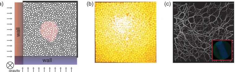
We study the biaxial compression of a granular monolayer on a nearly frictionless surface provided by an air table
(Fig.1). The system is composed of an inner subsystem (100
particles) and an outer bath (904 particles), which differ only
in the interparticle friction coeffcient. In particular, μ <0.1
for the subsystem andμ≈0.8 for the bath. The two systems
are both composed of a bidisperse mixure of disks (diameters
ds=11 mm anddl=15.4 mm) in equal concentrations.
At the beginning of each compression cycle, the system
is in a dilute (∼0.6), unjammed state unable to support
stress. Two walls then biaxially compress the system in a
series of small steps (=0.009, equivalently x =0.3
wall
wall
gravity
(c) (b)
(a)
mm or 0.02rl). After each step, the system is held in a single
configuration while measurements are made; this allows us to explore a series of static states prepared under increasing amounts strain.
For each configuration, a single CCD camera located above the apparatus records three separate images of the system: unpolarized white light for the particle positions, polarized light for recording the photoelastic response, and ultraviolet
light for identifying the subsystem particles, as shown in Fig.1.
Using the photoelastic image, we measure the normal and tangential forces at each contact on each disk in the assembly. To calculate the forces, we use a nonlinear least squares
optimization algorithm [45,46] to minimize the error between
the observed and fitted image of the particle. Details and source
code are available for download at [44]. The third image, taken
using a black-light illumination, identifies which particles are low friction via their fluorescent marking.
By repeating this protocol many times, we generate an ensemble of configurations for which we record particle
positions [Fig. 1(b)], and use photoelastic measurements
[Fig.1(c)] to calculate contact forces [44]. The presence of the
subsystem and bath allows us to characterize both the system as a whole, and to investigate the physical differences that exist between the high- and low-friction regions. In this paper, we focus on the force networks rather than the particles or their displacements. As the system is compressed via discrete, quasistatic steps, we observe the percolation of force chains
throughout both the bath and the subsystem at a valueJ. This
is the onset of rigidity, and as the system is further compressed beyond this point, the contact forces grow in strength and the average number of contacts per particle increases. For each
of the 97 configurations, we locateJ as the step at which
photoelastic signals are first present, and consider the changes to the mesoscale structure due to the subsequent applied strain steps. Further details of the experimental apparatus and
measurements were published previously [43].
Particle tracking
It is important to note that the construction of a multilayer network requires knowledge about which node (particle) is
which from one layer (strain step) to the next [41,42]. Under
the protocol described above, we are assured that no particles are removed from or added to the system, and we require that the multilayer network also has this constraint. (In general, multilayer graphs can indeed be constructed for growing systems, where the number of nodes is constantly changing.) In order to correctly identify the particles in each layer,
we use the Blair-Dufresne particle tracking algorithm [47].
This algorithm, implemented inMATLAB, requires the choice
of a “displacement” parameter, which is an estimate of the maximum distance that a particle moves between consecutive frames. As we do not expect large particle displacements in the jammed packings, we initialize the tracking with a displacement parameter value that is much less than the
minimum particle diameter ds, and increase the allowed
displacement in small increments until all particles are tracked consistently across all compressive steps.
III. MATHEMATICAL MODEL A. Multilayer network representation
In general,temporalmultilayer networks are mathematical
objects that describe and quantify the evolution of networked systems as a function of time or some other variable of interest
[41,42]. The construction of such a multilayer network first
requires a set of individual networks that describe the system at discrete time points, or steps. These static “layers” can
each be represented as an adjacency matrixA, describing the
connectivity and weight connecting the nodes in the given layer. The set of adjacency matrices may then be combined
into a rank-3 adjacency tensor A[48] to form a multilayer
network representation of the system. The elements ofAare
defined such that
Aij l= ⎧ ⎨ ⎩
aij l if nodeiandj are connected
in layerl,
0 otherwise,
(1)
whereaij l is the weight between nodesiandj in layerl, and
Lis the total number of layers (steps).
For the present situation, we are interested in how the force network of a granular packing reconfigures through a sequence
of compressive steps aboveJ. We thus represent the system
as an ordered, multilayer network, which captures the changes to the mesoscale structure as a function of compression. To form this network, we let nodes be particles, weighted edges be the forces between contacting particles, and the number of strain steps be the third dimension across which we observe changes in network structure. Using the force information obtained from the photoelastic disk experiments, we construct two multilayer force networks for a given experimental run,
one using the normal forcesFnbetween particles and another
using the magnitude of the tangential forces|Ft|. Specifically,
we denote the normal force adjacency tensor asAnij l, defined
as in Eq. (1) withaij l=fij ln, wheref n
ij l is the normal force
between particles i andj at stepl. Similarly, we write the
tangential force adjacency tensor asAt
ij l, defined as in Eq. (1)
withaij l= |fij lt |, wheref t
ij l is the tangential force between
particlesiandj at stepl. This process is repeated for all of
the experimental configurations, resulting in a large ensemble
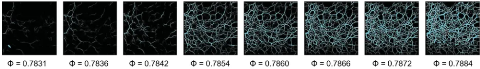
of multilayer networks. In Fig.2, we show an example set of
photoelastic images with the corresponding network of normal forces overlaid.
In addition to theintralayer weights, multilayer networks
have a second set of interlayer edges that connect nodes in
different layers of the network. In this study, we consider onlydiagonalandordinalinterlayer couplings, meaning that a given particle is connected only to itself (i.e., diagonal
cou-pling) and interlayer edges exist only betweenadjacentlayers
(i.e., ordinal coupling). The interlayer weights are crucial to
the structure of the network; in Sec.III B 4, we discuss how
these couplings are chosen for the granular system at hand. This graphical construction is a powerful approach. Importantly, each layer of the adjacency tensor encodes both the topology (connectivity) as well as the strength of interactions between particles in the system at a given
packing fraction. We will see that the extension to amultilayer
FIG. 2. The structure of the force network throughout compression. Photoelastic images of the system, taken at a sequence of eight steps aboveJ≈0.7825. The corresponding network of (normal) forces is overlaid on top of each picture. The collection of these static networks
are represented as a single multilayer network that captures the changes to the mesoscale structure throughout compression.
and characterization of the changes to the mesoscale structure throughout the compressive steps.
B. Community detection
A compelling reason to use graphical representations of
spatially embedded systems [49] is that network theoretic
approaches provide a means to extract and characterize organization that is present at a range of length scales. Granular materials are a prime example of a complex system in which multiple length scales are relevant to a full understanding of the system and to a prediction of bulk properties. For example, the fundamental interactions in these systems are local in the sense that they occur between nearest neighbor particles. But, under compression, those local interactions lead to important
heterogeneous structure at themesoscalein the form of force
chains [2–8,50].
In this study, we aim to both extract mesoscale structures from the force network, and then characterize the reconfig-uration that occurs in these structures due to the applied strain steps. In order to accomplish this, we build upon
recent approaches that utilizecommunity detectiontechniques
to extract groups of strongly interacting particles from the
granular network [26,40], generalizing the methods to the
multilayer regime.
Acommunityormodulein a network is a set of nodes that are densely interconnected amongst themselves, and relatively
weakly connected to other nodes [51]. The extraction of
community structure is of general interest in network science, as it is thought that these mesoscale units are important to
the function of many real systems [51]. Several community
detection methods exist [51,52]; here, we apply the popular
method of modularity maximization, whereby nodes are
partitioned into communities via maximization of a quality
function known asmodularity[53,54].
1. Single layer modularity maximization
In a single layer network with adjacency matrix A,
modularity is given by
Qsing=
1
2m
ij
[Aij−γ Pij]δ(ci,cj), (2)
whereci is the community of nodei,cj is the community of
nodej,Pij is the expected edge weight between nodesiandj
under a specified null model, andγis thestructural resolution
parameter. In the overall normalization,m=1 2
ijAij, which
is the weighted degree or strength of the network. The
structural resolution parameter γ allows for the control of
size and number of communities: smaller γ leads to larger
communities, and larger γ leads to smaller communities.
Maximization ofQsingwith respect to the assignment of nodes
to communities yields a partition in which intracommunity connections are as strong as possible relative to the null model. It is important to note, however, that modularity maximization
is NP hard [55] and should therefore be repeated several times
for the same network and set of parameters in order to obtain
an ensemble of optimizations [56]. Throughout this work, we
use a Louvain-type locally greedy algorithm for modularity
maximization [57,58].
2. A physically informed null model
A proper choice of null model is vital to community detection techniques, as it affects both the interpretation and
utility of the community structures obtained [56,59]. The
most commonly used null model in the literature is the
Newman-Girvan (NG) model [53,54], which in the case of
a static network is given by Pij =
kikj
2m, where ki=
jAij
is the strength of nodei, and mis the total strength of the
network, as before. In the Newman-Girvan model (which is
also sometimes referred to as the configuration model),Pij
gives the expected edge weight between nodes i and j in
a randomized network that has the same degree distribution as the real network. As a randomized version of the real graph, the NG model is most appropriate to use as a null model in situations where all connections between nodes are
at least possible. In many physical or spatially embedded
systems, however, this is not the case, and there are constraints that prevent the existence of several edges. For example, in the granular networks considered here, edges can only exist between nearest neighbor particles, and it is imperative to consider this fact when designing a null model for these types of systems. A better choice in this instance is the physically
informedgeographic null model[40,56], defined to be
Pij = fBij, (3)
wherefis the average interparticle force (either normal or
tangential) in the network andBij is the contact matrix, with
elements
Bij =
1 if particleiandj are in contact,
0 otherwise. (4)
Because this null model maintains the contact structure of the real network, it importantly takes into account the physical constraints on the possible patterns of connectivity between particles. Additionally, it selects for strongly connected sets of
FIG. 3. An example of single layer community structure. When single layer community detection is performed on the series of normal force networks aboveJ, the groups of particles at each step correspond to force chain structures. However, there is no notion of linking these
mesostructures from one compressive step to the next.
3. Multilayer modularity maximization
When community detection is performed on a series of single layer granular networks, such as those obtained here
after each applied strain step, the result is a set ofindependent
partitions of particles into communities at each step (Fig.3).
As demonstrated in [40], the communities at a given step
correspond to the physical force chains observed in the photoelastic disk experiments. However, in this scheme, the community structure is not in any way linked from one layer to the next, barring any notion of continuation. Instead, the communities are treated as independent from one another, which is an inaccurate representation of the physics and further challenges our ability to directly capture the evolution of network structure and reconfiguration at the mesoscale.
To form a more complete picture of the changes in network architecture, we investigate the community structure ofmultilayergranular force networks by applying the recent generalization of modularity maximization to temporal
net-works [60,61]. In this formulation, the multilayer modularity
is defined to be
Qmulti= 1
2μ
ij lm
[(Aij l−γlPij l)δlm+ωj lmδij]δ(cil,cj m),
(5)
whereAij l is the (i,j) component of the adjacency tensor in
layerl,Pij l is the (i,j) component of the null model tensor
in layer l, andγl is the structural resolution parameter for
layerl. In addition toγ, the multilayer modularity requires
another free parameterω (often referred to as aninterlayer
couplingortemporal resolution parameter) which sets the the
strength of connections between layers. Namely,ωj lm is the
strength of the coupling that links nodej in layerlto itself in
an adjacent layerm(i.e., the diagonal and ordinal coupling).
The quantitiescil andcj mare the community assignments of
nodeiin layerland nodej in layerm, respectively. Defining
the intraslice strength of nodej in layer l as kj l=
iAij l
and the strength of nodej across layers aswj l=
mωj lm,
then the multilayer strength of node j in layer l is given
by κj l=kj l+wj l. Finally, in the overall normalization, μ
is the total strength of the adjacency tensor A, given by
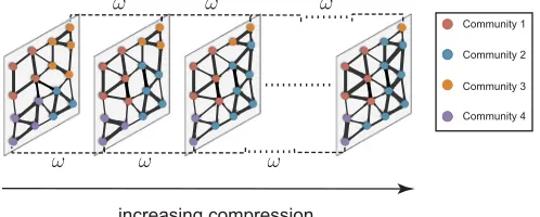
μ= 12j lκj l. In Fig.4, we show a schematic of a multilayer
granular force network with evolving community structure. Importantly, the communities can persist across all layers and we can track their reconfiguration in terms of particle content and strength throughout the series of strain steps.
As in the formulation ofQsing, the choice of null model
inQmulti is an important one, particularly when considering
systems with strict constraints on the allowed connectivity between nodes. For granular networks, we generalize the
ge-ographic null model to the multilayer regime. For community detection on the normal force network we use
Pn ij l = f
n
lBij l, (6)
where fn
l is the average of the normal component of the
interparticle forces at compressive steplandBij lis the contact
matrix at compressive stepl. For the tangential network, we
take the null model to be
Pt ij l = |f
t|
lBij l, (7)
where |ft|
l is the average of the absolute value of the
tangential component of the interparticle forces at compressive stepl, andBij lis the contact matrix at that step.
In each layer, we normalize the force network (Anij l or
|At
ij l|) by the mean interparticle force in the corresponding
layer. Thus, after normalization we havefn
l=1 in Eq. (6)
and|ft|
l=1 in Eq. (7), for alll. This normalization ensures
that the community structure is not purely driven by the final layer, which will have the largest total edge weight due to it being the most compressed.
Community 1 Community 2
Community 3 Community 4
increasing compression
4. Choosing omega: Flexibility as a measure of network reconfiguration
The two parameters in the multilayer modularity quality
functionωandγ must be chosen by the investigator. Recall
that the structural resolution parameterγ regulates the size
and number of detected communities; in this study, we use
γl ≡γ =1 for alll. As can be seen from Eqs. (5)–(7), the
physical meaning of this value is that it selects for communities within each layer that have stronger than average force. The
choice ofωis an active area of investigation; currently, there
is no consensus in the literature on a single, broadly applicable method to determine the interlayer coupling. In this work, we make a physically informed choice. As described in the
previous section, ω is in general a tensor that can take on
different values between each layer or for different nodes. Since to our knowledge this is the first study on multilayer granular networks, we begin by taking the simplest case
of a scalar interlayer coupling, choosing ω to be the same
for all particles and all pairs of layers, such thatωj lm≡ω
for allj,l,m. However, it is important to point out that the
interlayer coupling could be different for different particles. For example, one could alternatively tune the relative value
of ω for a given particle based on a particle property.
Investigation of more complicated methods for choosing the interlayer couplings may be an interesting direction for future work.
To proceed, it is necessary to understand the effect ofω
on the community structure. There are two limiting cases
which are relatively simple to grasp: whenω=0, there are
no connections between layers of the adjacency tensor, and we therefore recover the results of static community detection
(Fig.3). At the other extreme,ωcan be made large enough such
that the strength ofinterlayerconnections entirely overwhelms
the strength ofintralayerconnections, resulting in completely
consistent community structure across all compressive steps
(that is, no observable changes; see Fig.18in the Appendix for
an example partition at largeω). To understand what occurs
in-between these limiting cases, we consider a simple measure
of network rearrangement calledflexibility, or, previously
defined in [62]. The flexibility of a single particle i, ξi, is
given by
ξi = gi
L−1, (8)
wheregi is the number of times that the particle changes its
community and L is the total number of strain steps. The
flexibility of the entire multilayer network is then given by the mean flexibility of all particles
= 1
N
i
ξi, (9)
whereNis the number of particles.
In order to choose a physically relevant value of the interslice coupling, we run 20 optimizations of multilayer
community detection on the normal force network An for
each packing, for several values of ω between 0 and 1, in
steps of ω=0.01. Note that ω=0.01 corresponds to a
coupling which is equal to 1
100 of the mean edge weight in
0 0.2 0.4 0.6 0.8 1
0 0.2 0.4 0.6 0.8 1
average flexibility over packings,
interlayer coupling,
0.14 0.16 0.18 0.2 0.22
0 5 10 15 20 25
number of packings
optimal ω value
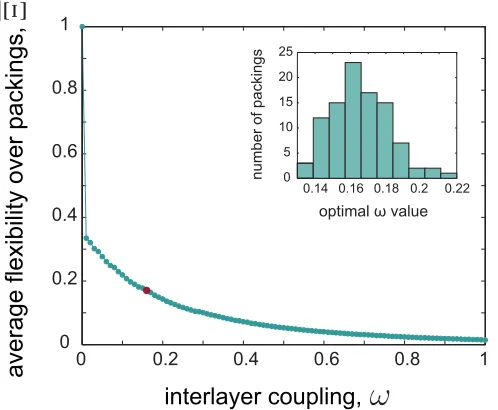
FIG. 5. Choosing an optimal interlayer coupling. The average network flexibility is governed by the value of the interlayer coupling ω. Each dot is the average of network flexibility over all experimental packingsvs the interlayer couplingω. Whenω=0,=1 and the results of static community detection are recovered; there is no persistent structure across compression. When ω=1, ≈0 and the particle contact forces within each layer are overwhelmed by the weight of the interlayer coupling such that the community structure exhibits complete consistency throughout the compressive steps. Atω=0.01,max≈0.3349. The optimal interlayer coupling ω∗=0.16 is denoted by the red dot, and is chosen such that (ω∗)≈max/2. This ensures a balance between intralayer and interlayer weights. The inset shows what the distribution of ω∗
would be if the identical procedure were performed for each packing individually.
a given layer, due to the normalization procedure described
in Sec. III B 3. Due to the stochastic nature of modularity
maximization [55], we avoid an interlayer coupling close to
zero, as the community structure is more likely to be influenced
by noise in the algorithm. At each ω, we compute for
all optimizations of a given packing, and then average over optimizations to obtain a single value of flexibility for the
packingopt. In what follows, we will denote averages over
optimizations as. . .opt, and averages first over optimization
and then over packings with an overbar.
As shown in Fig. 5, we observe that away from ω=0,
the average flexibilitydecreases smoothly as the interlayer
coupling increases (and see Fig.16of the Appendix for the
plot of Qmulti versus ω). As expected, right at ω=0, the
network flexibility is unity, indicative of the fact that there is no consistency in community structure across layers. That is, at each step all particles are assigned to new communities which are independent from the community they were assigned
to in the previous step. Atω=1, which corresponds to an
Interestingly, at the first ω value away from zero,
sharply drops to≈0.33. The presence of this steep decline is
explained by a recent mathematical result, which demonstrates
that the case ω=0 is singular in the sense that even when
ω=with 0< 1, there will be at least some persistent
community structure [61]. Furthermore, the mathematics
behind this finding are independent of the particular system or multilayer network being studied. We thus take the value
of obtained from the first small step away from 0 at
ω=0.01 to be the upper bound of network flexibility,max;
from that point forward, smoothly decreases to zero (see
Appendix B for further considerations into this point). To
further characterize the behavior of the flexibilityversus ω
curve, we assessed whether the trend could be described
as exponential decay, such that for each opt, we have
opt≈Ae−ω/ωo. We find that the data can indeed be well
approximated by an exponential. Theωofor all packings fall
in the range 0.26ωo 0.40, and represent characteristic
interlayer couplings for the system.
Atωvalues too far into the exponential tail, the
communi-ties will not be sensitive to the structure present within a given
layer, and at small values of ω, dependence on the specific
ordering of layers becomes less important. We thus pick the
optimal value of interslice couplingω∗ to be the value such
that(ω∗) is approximately half of the maximum flexibility
max. This procedure yields a value of ωthat balances the
tradeoff between the importance of intralayer edges (particle contact forces) and persistent structure across network layers.
In Sec.IV C, we further validate this choice by comparing
the community structure obtained atω∗ to three null models,
showing that in each case, the real network is distinguishable from the null model.
Using the method described above, we find ω∗=0.16
(denoted by the red dot in Fig. 5), and we use this value
in community detection for all packings and for both the
normal and tangential force networks. The inset of Fig. 5
shows what the distribution of ω∗ would be if we were to
optimize ω for each packing individually. We acknowledge
that there are several other methods that could be used to determine an appropriate coupling, but here we have focused
on a straightforward method to choose a physically meaningful
ω, which yields intermediate values of network flexibility.
In the Supplemental Material available online, we examine the robustness of several of the results detailed below to variations in the interlayer coupling around the optimal value [63].
IV. RESULTS
A. Extraction of mesoscale structure from the multilayer force network
To extract pressure dependent particle assemblies (commu-nities) from the multilayer force networks of each experimental
run, we maximize multilayer modularity [Eq. (5)]. We consider
both the normal and tangential force networks separately, with
Aij ldefined as in Sec.III A, andPij lgiven by Eq. (6) [or (7)].
As determined in the previous section, in both cases we use
γ =1 and ω=ω∗=0.16. For each particle configuration,
we carry out 20 maximizations of the multilayer modularity to obtain an ensemble of partitions, each with their respective value ofQmulti.
By the nature of modularity maximization and our choice of null model, the resulting communities correspond to spatially localized, mesoscale groups of particles that display collective organization throughout the compression process. In particu-lar, the first term of Eq. (5) selects for groups of particles carry-ing above average force and that are geographically nearby, and the second term allows those groups to be consistently tracked
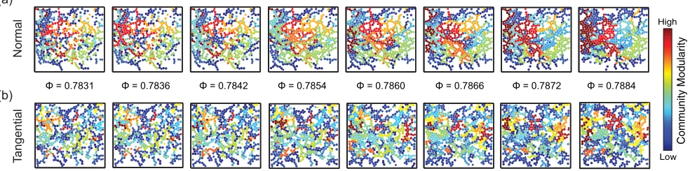
between steps. In Fig.6, we show an example of the community
architecture at each step aboveJ detected from the normal
force network [Fig. 6(a)] and the tangential force network
[Fig.6(b)], of a particular experimental configuration. In both
cases, communities are colored according to their multilayer
modularity valueQmulti. Importantly, the same color at each
strain step corresponds to the same community, to provide a visual sense of how particle assemblies are linked continuously throughout compression. Unlike in single layer modularity maximization, the communities here can persist across layers and are dependent on their history. This formalism thus
Community Modularity
Low High
Φ = 0.7842 Φ = 0.7854
Φ = 0.7831 Φ = 0.7836 Φ = 0.7860 Φ = 0.7866 Φ = 0.7872 Φ = 0.7884
Normal
T
angential
(a)
(b)
FIG. 6. Multilayer community structure of a compressed granular packing. For both the normal (a) and tangential (b) networks, particles are shown at their actual locations in physical space, and are colored according to their community assignment. Redder colors correspond to communities with higher multilayer modularity. The packing fraction increases from left to right, and only the steps with > Jare shown.
provides a means to directly examine how the force network evolves and reconfigures under compression.
It is important to point out that the structure uncovered with multilayer community detection is representative of the system as a whole across all layers, and not necessarily of the
static force chain structure of individual layers (unlessω=0).
Because of this, it is not required that a community in a given layer consists of only physically connected particles; rather, communities in a given layer are dependent on the structure of the entire multilayer network as a whole. In this way, the communities embody the changing network architecture and are a consequence of the evolving stress pattern; we thus observe the breakup and coalescence of communities across the applied compressive steps. The normal and tangential networks exhibit some similar features, but there are also clear differences. In both cases, the communities become more compact with pressure, but these structural patterns are most clearly evident for the normal force network. The length scale of communities from the tangential network is also smaller than those extracted from the normal forces. In the following sections, we study the reconfiguration and physical properties of this architecture, and quantify these differences between the normal and tangential mesostructures.
B. Characterization of mesoscale reconfiguration
We characterize the changes to the mesoscale structure of the multilayer community structure using two diagnostics:
network flexibility [Eq. (9)] and community stationarity
ζc. Recall that the network flexibility quantifies the amount of
reconfiguration in the network at the particle level, as measured by the fraction of steps over which a particle changes its com-munity allegiance. As a second measure of reconfiguration in the stress pattern, we also consider the community stationarity
[56,64], which measures the consistency of particle content in
each community throughout compression.
To define stationarity, we begin by writing the autocorrela-tionJ(cl,cl+m) between a given community at layerl,cl, and
the same community at layerl+m,cl+m, as
J(cl,cl+m)=
|cl∩cl+m|
|cl∪cl+m|
, (10)
where |cl∩cl+m| is the number of particles present in
communitycat strain steplthat arealsopresent in community
c at step l+m, and |cl∪cl+m| is the number of distinct
particles present in communitycat strain steplorstepl+m.
Then, ifli is the layer in which community cfirst appears,
andlf is the layer in which it last appears, the stationarity of
communitycis
ζc=
l=lf−1
l=li J(cl,cl+1) lf−li
. (11)
In this way, communities that experience large changes in their particle content over consecutive compressive steps will have
larger values of ζc than communities with more consistent
structure. The average stationarity of a multilayer network is
obtained by taking the mean ofζcover allnccommunities:
ζ = 1 nc
c
ζc. (12)
0.12 0.16 0.2 0.24 0.28
0.55 0.6 0.65
0.7 0.75
0.8 0.85
Flexibility, Ξ
Normal Tangential
Stationarity, ζ
Normal Tangential
(b) (a)
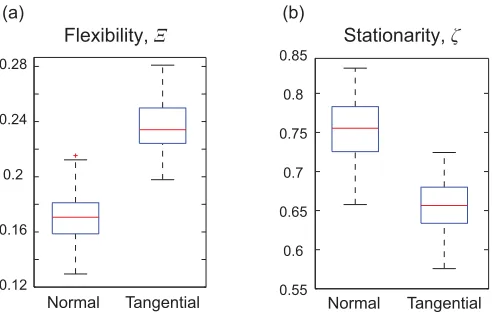
FIG. 7. Measures of multilayer community structure for the nor-mal and tangential force networks. The structure and reconfiguration of the community structure of the normal and tangential force networks is characterized by (a) network flexibilityand (b) network stationarityζ. The boxplots are constructed by averaging statistic values over optimization for each experimental packing. The red line then denotes the median over packings and the edges correspond to the 25th and 75th percentiles. For the same interlayer coupling, the normal and tangential networks have statistically different behavior in terms of these measures of network reorganization.
In Fig.7, we show boxplots over the particle configurations
ofandζ for the normal and tangential force networks. We
have averaged these diagnostics over the 20 optimizations,
to obtain a mean value of opt andζopt for each
experi-mental packing. For the stationarity calculation, we exclude
singletoncommunities, which only contain one particle in all layers.
We test whether the observed changes to the normal and tangential force networks can be distinguished by per-forming nonparametric permutation tests on the flexibility and stationarity values. For the network of normal forces,
there are 97 values of the flexibility nopt and stationarity
ζnopt(one for each laboratory configuration). Repeating the
same protocol for the tangential forces yields another set
of values topt andζtopt. We calculate the difference in
the means of these two distributions, and test whether that difference is greater than expected in the null distribution created by reassigning statistics uniformly at random to the two groups: “normal” and “tangential.” Using this test, we find significant differences in the means (over optimizations
and then packings) of both statistics, with bothpvalues less
than 1×10⁻³. In particular,n< t andζn> ζt. From this
finding, we conclude that at the same value of interlayer coupling, the multilayer network of normal forces tends to exhibit less reorganization during compression than the network of tangential forces. This sensitivity to differences in two related but distinct force networks suggests that our method may be more broadly applicable. For example, it could be used to test for differences and classify different types of granular systems composed of varying particle materials, shapes, or sizes. In the Supplemental Material, we show that this distinguishability is robust to variations in the interlayer
C. Reconfiguration of network architecture during compression: A null model comparison
Perhaps more important than absolute values of network measures is whether or not the network evolution observed in the real, physical system is significantly different than what is expected from relevant null models, and whether or not our model is sensitive to these differences. In this section, we demonstrate that the multilayer community structure of the compressed granular configuration is indeed distinct from three null models with respect to the diagnostics defined
previously ( and ζ). Here, we additionally consider the
multilayer modularityQmulti. (Recall thatQmulti is a general
measure of how well the network can be partitioned into densely interconnected groups of particles throughout the compression process, with respect to the physically appropri-ate geographic null model.) To ensure a fair comparison, we test the real force networks from each of the 97 experimental realizations against null models that are built using the force information from the same experimental run. Furthermore, we analyze the normal and tangential forces separately. To determine statistical significance, we perform permutation tests; assignments of statistic values to the two groups, “real network” or “null network,” are permuted uniformly at random to construct a null distribution of expected differences between the two distributions.
In the first case, we impose the elimination of steady perturbation on the system, comparing the real multilayer force networks to null models built by setting all layers to be equal
[Fig.8(a)]. In particular, we construct a null networkArepeat
by repeating the real force network at a constant layers,L
times (recall thatL is the total number of layers). Carrying
out this process for all such constant layers yields a set ofL
null networks for each packing. We run community detection 20 times for each null network, and compute the network diagnostics (Qnullmulti,null, andζnull) for each trial. We average
quantities first over the optimization realizations, and then over the different networks. Physically, this simple null model serves as a control that allows us to assess the implications and consequences of compression on the detected community structure. Since there are no changes in topological structure or edge weights from one layer to the next in the synthetic networks, we expect all changes in community structure to be due to noise. This baseline network reconfiguration should be much less than the reconfiguration that occurs in the real networks, which encode the compression procedure. Indeed, for both the normal and tangential force networks, we see that the null models have significantly lower flexibility,
null< real, and higher stationarity, ζnull > ζreal, than the
compressed system [see Figs.8(a),8(d), and8(g)]. Note also
that the modularity of the null model is greater than that of the true networks, which is also expected since the null models will be partitioned into highly consistent community structure across layers.
We next compare the real system to a null modelAlayers,
constructed by permuting the layers (strain steps) of the real
networks uniformly at random [Fig.8(b)]. In the experimental
protocol, compression is applied systematically, in small and always increasing steps. The null model considered here effectively eradicates this regularity in the layer ordering.
The expectation is that the real networks will have less restructuring than the scrambled model. For each experimental packing, we create 20 null networks built from different random permutations of the layers, and run 20 optimizations of the Louvain algorithm for all permutations. As before, we compute null,ζnull, and Qnullmulti, and average the results first
over optimizations and then over permutations. In Figs.8(e)
and8(h)we compare the real system to the null model, finding
that our method is again sensitive to differences in the changing mesoscale organization of the real and synthetic networks. For
both the normal and tangential force networks,null> real,
andζnull< ζrealimplying more steady and regular progression of community structure in the real system. In addition, we observe a slight decrease in modularity in the layer permuted normal force network, suggesting that the real compression protocol yields stronger multilayer community structure. The modularity of the tangential forces is less affected by layer scrambling than that of the normal forces. We also find that the real system can be distinguished from this null model with respect to an alternative measure of network reconfiguration
known as promiscuity, [65]. See Appendix C 2 for a
definition of this statistic and the results of the null model analysis.
In the final null model [Fig.8(c)], we consider the spatial
distribution of forces throughout the system. We construct a
null modelAedges by permuting the edge weights uniformly
at random within each layer while maintaining the original contact topology and ordering of slices (for a related but
distinct null model, see [28]). It is known that the organization
of interparticle forces is crucial for the stability of granular packings. This fact is manifested in force chains, branching groups of particles that bear the majority of the load in the system. Therefore, for the multilayer model to be useful, it should not be agnostic to the pattern of forces present in phys-ically realizable systems. For each of the 97 configurations, we form an ensemble of null networks by permuting the forces uniformly at random within each layer 20 different times, and then optimize modularity 20 times for each permuted network. As before, this is done separately for the normal and tangential forces. In this case, we expect the synthetic networks to display more reconfiguration and less modular structure than the physical networks. We observe that the diagnostics of multilayer community structure are highly distinguishable between the real multilayer force networks and the null
model [Figs.8(f)and8(i)]. In particular, the force-permuted
networks exhibit more flexibilitynull> real, less stationarity
ζnull< ζreal, and decreased modularity Qnull
multi< Qrealmulti for
both the normal and tangential components. These results confirm that the network structure of the real system is less variable and undergoes less reorganization, and that the modularity is stronger, compared to the null model. In
Ap-pendixC 2, we additionally show that these results hold for the
promiscuity.
The findings presented in this section crucially demon-strate that the multilayer network model and community detection are sensitive to differences in the evolution of the stress pattern of the compressed system compared to three
relevant null models, with respect to , ζ, and Qmulti. In
Repeat Same Layer Permute Layer Order Permute Edge Weights
Null
Models
(c) (b)
(a)
−0.5 0 1
Qmulti
Ξ ζ
(d)
Normal Force
Real - Null
Real
0 1
Qmulti
Ξ ζ
(g)
−0.8
Tangential Force
Real - Null
Real
−0.25 0 0.15
Qmulti
Ξ ζ
(e)
−0.08 0 0.08
Qmulti
Ξ ζ
(h)
−0.25 0 0.25
Qmulti
Ξ ζ
(i) 0.3
−0.8 0
Qmulti
Ξ ζ
(f)
p = < 10-3 p = < 0.05 * **
** ** **
** ** **
** ** **
** ** **
** ** *
** **
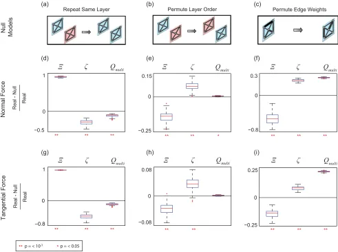
FIG. 8. A comparison of the multilayer granular networks to three null networks. The community structure of the multilayer granular system is compared to three null models (top row), using the quantities,ζ, andQmulti. For each null model, the boxplots show the normalized difference between the real and null network diagnostics for all experimental configurations, and for the normal (second row) and tangential (third row) components. Significant differences between the real and null networks exist when the boxplots are above or below the zero line. Thepvalues obtained from permutation testing are shown beneath each box to quantify the significance of results. (If nopvalue is shown, the difference is not significant). (a) A null model formed by repeating the same layer for all steps,Arepeat. The values,ζ, andQmultiare statistically different between the real and null networks for the normal (d) and tangential (g) components. (b) A null modelAlayers, constructed by permuting the ordering of layers uniformly at random. The values,ζ, andQmultiare statistically different between the real system and null model for the normal forces (e), andandζare statistically different between the real system and null model for the tangential forces (h). (c) The third null modelAedgesis built by permuting the edge weights uniformly at random, while maintaining the original contact topology and layer ordering. The values,ζ, andQmultiare statistically different between the real and null networks for both the normal (f) and tangential (i) components.
and weights, scrambled layers, or scrambled edge weights (but same topological structure). Even more importantly, the differences in the reconfiguration agree with what is expected from a physical standpoint, making evident the powerful utility of this framework.
D. Physical properties of multilayer mesostructures
In the previous section, we examined three measures to quantify the community structure of the multilayer granular network. However, the diagnostics we considered did not directly describe changes in the physical properties of the mesoscale organization. We turn now to a physical description of the network architecture, and define measures to quantify the size scale, strength, and geometry of community structure
throughout compression. We then ask whether the physical properties of mesoscale particle assemblies can be related to the measures of force network reorganization previously defined.
1. Progression of community-level features throughout compression
We characterize the physical nature of community
struc-ture with three measures: size, strength, and sparsity, and
examine how these quantities change throughout compression. Similarly to the previous section, we consider, compare, and contrast both the normal and tangential force networks. The sizesc
l of communitycat strain stepl is simply the number
strength of a community at layerlas σlc, and define it to be the average amount of force (normalized by the mean force in
the layer) on a particle in communitycfrom intracommunity
contacts. Mathematically,
σlc= 1 sc l
i,j∈cl
Aij l, (13)
where A is either the normalized normal or tangential
force network. Finally, we consider a measure of spatial
compactness, which we term the community sparsityηc. The
sparsity of a community is closely related to thehull ratio,
which has been defined and used to quantify the geometric
arrangement of compressed particle assemblies [66]. The hull
ratiohc
l of a community at strain steplcan be understood as
the ratio of the areaaof particles in the community to the area
of the convex hull of the groupahull, such that
hcl =
i∈clai
ahull , (14)
where the area of particleiisai =π ri2, withriequal to the
par-ticle radius. We then take the community sparsity at layerlto be
ηcl =1−hcl. (15)
With this definition, small values ofηcorrespond to spatially
dense groups of particles, and high values ofηcorrespond to
sparse particle configurations.
We now use each of these physical characteristics to quantify the progression of mesoscale community structure throughout the compression process. Given a partition of particles into communities, we computeslc,σlc, andηlcat each
strain step l, for all communities except those which have
sc
l =1 for all l (i.e., they are always singletons). We then
define sl,σl, andηl to be the average over all communities
present in layerl:
sl=
1
ncl
cl
slc, (16a)
σl =
1
ncl
cl
σlc, (16b)
ηl =
1
ncl
cl
ηcl, (16c)
where ncl is the number of communities present in layer l.
Repeating this process for all community detection optimiza-tions and all particle configuraoptimiza-tions, we form representative curves of each physical quantity as a function of strain step by averaging the measures defined above first over optimizations and then over experimental configurations. We denote the final averaged physical quantities for size, strength, and sparsity as ¯
s, ¯σ, and ¯η, respectively.
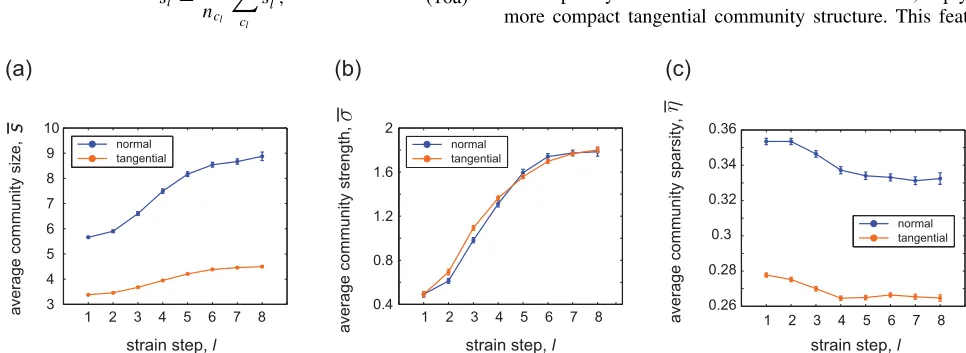
We first observe that the size of the mesoscale structure
increases smoothly as a function of the strain steps [Fig.9(a)],
suggesting an increasing scale of mesostructure organization with compression. However, the normal force communities are noticeably larger in size, and undergo relatively more growth throughout strain steps than the communities from the tangen-tial network. These differences imply that the communities from the network of normal forces are characterized by a larger characteristic size scale than those of the tangential force net-work, and that the normal force network responds differently to increasing pressure. Some of these features are partially recognizable by eye in comparing the community structure in
Figs.6(a)and6(b). We also find that the community strength
increases smoothly over the applied strain steps, for both the normal and tangential components. This behavior signifies the mesoscale architecture becoming more strongly connected throughout compression, which agrees with the physical
expectation. Note that the average community strength ¯σ was
computed on the normalized networks (see Sec. III B 3),
which explains the similar scale between the normal and tangential curves. Finally, we observe a slight decrease in community sparsity across strain steps, especially during the beginning stages. In addition, the tangential network displays lower sparsity than that of the normal force network, implying more compact tangential community structure. This feature
1 2 3 4 5 6 7 8 3
4 5 6 7 8 9 10
normal tangential
average community size,
(a)
strain step, l
1 2 3 4 5 6 7 8 0.4
0.8 1.2 1.6 2
average community strength,
(b)
1 2 3 4 5 6 7 8 0.26
0.28 0.3 0.32 0.34 0.36
average community sparsity,
(c)
normal tangential
normal tangential
strain step, l strain step, l
TABLE I. Percentages of communities from the network of normal forces that exhibit linear trends with respect to strengthσor sparsityηthroughout compression. The numbers reported correspond to averages over optimizations and packings, and errors are the standard errors of the mean.
Trend Strengthσ Sparsityη
Increasing 32.8±0.6 12.2±0.3
Decreasing 3.8±0.3 42.3±0.8
is likely tied to the smaller size of tangential communities, which constrains the set of possible spatial arrangements of the particles within a community.
2. Trends in physical characteristics are diverse
In addition to quantifying the average behavior of mesoscale architecture, it is also important to investigate the behavior of individual communities throughout compression. Although it is possible that all communities progress similarly to the average behavior of the system (for example, coalescing to create communities of increasing size and strength, but decreasing sparsity), this does not have to be the case. We find, in fact, that the situation is quite the opposite; at the level of single communities, the progression of physical structure varies greatly. We demonstrate this in a simple way. First, we identify the number of communities that exhibit linear trends with respect to size, strength, or sparsity as a function of strain
step. TablesIandIIshow the results of this analysis for the
normal and tangential networks. We observe that the majority
of mesostructures do not exhibit consistent and predictable
linear trends in terms of their physical properties throughout the compression process. While some linear tendencies are much more likely to occur than others (for example, increasing strength and decreasing sparsity), the behavior of many communities cannot be characterized by a simple linear relationship. This result highlights the important diversity of mesoscale structural evolution.
Next, we ask if and how the set of communities which
do have linear behavior with respect to a given physical
property, are related to each other. In Fig. 10, we plot the
slope of the linear regression fit of sparsity versus the slope of strength, for each community in all optimizations and experimental packings. Again, the scatter plots point to the variation of mesostructure development, as all quadrants (with the exception of the upper left) are significantly filled in. These data support the notion that communities may coalesce,
TABLE II. Percentages of communities from the network of tangential forces that exhibit linear trends with respect to strengthσor sparsityηthroughout compression. The numbers reported correspond to averages over optimizations and packings, and errors are the standard errors of the mean.
Trend Strengthσ Sparsityη
Increasing 18.3±0.3 14.9±0.3
Decreasing 2.3±0.1 28.1±0.6
(a)
(b)
FIG. 10. Scatter plots demonstrating the diversity of multilayer community structure. The relationship between the slopes of commu-nities that exhibit linear trends with respect to strength and sparsity across compression. For both the normal (a) and tangential (b) force networks, all but the upper left quadrant are quite populated, pointing to the diversity in how the community structure changes throughout the compression process.
disband, or become increasingly branchlike, and each of these behaviors is observable as the force network reorganizes under compression.
To quantify the codependence of the two statistics, we first find the number of communities (i.e., the intersection) that fall within each quadrant for each optimization and packing. For
example, ifσ↑ are the communities with linearly increasing
strength andη↑are those with linearly increasing sparsity, then
we compute the number of communities that satisfyσ↑∩η↑
(upper right quadrant of the scatter plots). Then, to determine
how often increasing strength (σ↑) occurs with increasing
sparsity (η↑), for example, we normalize the intersection by the
total number of communities withσ↑. Conversely, if we want to
know the percentage of communities with increasing sparsity
instead divide the intersection by the number of communities
inη↑. TableIIIin AppendixC 1shows the percentages for each
of the possible combinations. The strongest relationship occurs
between communities withσ↓andη↓. In this case, we find that
if a community has linearly decreasing strength with strain step, then it is likely to also be more compact (but note that not many communities decrease in strength in the first place). These results may be due to the community losing particles and thus becoming more dense [on average for the normal
(tangential) network, 98.6% (96.6%) of communities with
linearly decreasing strength and sparsity also have linearly decreasing size]. The nearly empty upper left quadrants are consistent with this relationship as well; communities with decreasing strength rarely become more spatially spread out throughout compression. We also find that on average, more than half of the communities with increasing sparsity also have increasing strength, which is likely due to the community gaining particles, thus allowing it to take on configurations which are more spatially extended [on average for the normal
(tangential) network, 93.9% (91.7%) of communities with
linearly increasing strength and sparsity also have linearly increasing size].
E. Linking physical properties to network reconfiguration
Thus far, we have independently characterized the mul-tilayer community structure using notions of network reor-ganization (flexibility and stationarity), and using physical quantities, (size, strength, and sparsity). We now attempt to link these two ideas together, asking whether network reconfiguration can be related to physical aspects of the packing structure.
1. Local reorganization
We first investigate the relationship between particle
flex-ibilityξ [Eq. (8)] and the interparticle force f. Recall that
ξ is a measure oflocalreconfiguration in the force network
in that it is defined for a single particle, but it is determined
from themesoscalecommunity structure. For every multilayer
community partition, we compute the flexibility of each
particle as given in Eq. (8), and average these values over
partitions. This yields a single value of flexibilityξifor theith
particle in a given experimental run. We do this for the normal and tangential force networks separately.
Our first finding is that flexibilityξ is strongly correlated
with the average force on a particle throughout strain steps
fφ, as well as the average absolute change in force on
the particle |f|φ between consecutive strain steps. This
result holds for both the normal and tangential components.
For theith particle, the average change in force |fi|
φ is
given by
|fi|φ =
1
L−1
l=L−1
l=1
fli+1−fli, (17)
where fli is the total force on the ith particle in layer l,
determined from the adjacency tensor asfli=jAij l.
In particular, we observe that particles with high flexibility
ξ also tend to have high values of average force fφ and
average change in force|f|φ. In Fig.11, we plotξ versus
0 0.04 0.08 0.12 0.16 0.20 0
0.2 0.4 0.6 0.8 1
0 0.04 0.08 0.12 0.16 0
0.2 0.4 0.6 0.8 1
Normal Force Network Tangential Force Network (a)
(b) (d)
(c)
particle flexibility
,
0 0.2 0.4 0.6 0.8 1.0 1.2 1.4 1.6 1.8 0
0.1 0.2 0.3 0.4 0.5 0.6 0.7
0 0.1 0.2 0.3 0.4 0.5 0.6 0.7 0
0.1 0.2 0.3 0.4 0.5 0.6 0.7
average absolute change in force on particle, average force on particle,
particle flexibility
,
particle flexibility
,
particle flexibility
,
average force on particle,
average absolute change in force on particle,
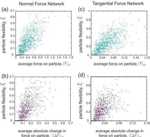
FIG. 11. Force drives local network reorganization. (a), (c) Scatter plots of particle flexibilityξ versus the average force on a particle across compressionfφ for a sample packing. In both the
normal and tangential networks, there is a strong, positive Spearman correlation between the two quantities. (b), (d) Scatter plots of particle flexibility ξ versus the average absolute change in force on a particle across compression|f|φ for a sample packing. In
both the normal and tangential networks, there is a strong, positive Spearman correlation between the two quantities. (See Fig.22for the distribution of correlations for each packing.)
fφ for each particle using the normal [Fig. 11(a)] and
tangential [Fig. 11(c)] force networks of one experimental
configuration. Figures11(b)and11(d)showξversus|f|φ.
We quantify these relationships for all experimental packings
using the Spearman’s rank correlation ρ. For the normal
forces, the average correlations over packings for ξ versus
fφ andξ versus |f|φ are ρf =0.81 and ρf =0.74,
respectively, with all p values satisfying pf <1×10−174
andpf <1×1−127, respectively. [In Figs.22(a)and22(b)
of the Appendix, we show the distributions of ρf andρf
for all packings.] For the tangential forces, ρf =0.80 and
ρf =0.71, with allpvalues satisfyingpf <1×10−181and
pf <1×10−109. [In Figs.22(c)and22(d)of the Appendix,
we show the distributions of ρf and ρf.] In addition to
the flexibility, we also tested the relationship between force and reconfiguration on a more robust measurement of local
network rearrangement called promiscuity[65], finding that
the relationship still strongly holds. See Appendix C 2for
a description of the promiscuity statistic, an example scatter plot, and correlation values.
To understand these results, first recall that the flexibility of a particle is a measure of how strongly fixed the particle
is to its given community;ξ is the number of times a particle
changes community normalized by the number of possible
changes, so lower values of ξ correspond to particles that