EXACT: Explicit Dynamic-Branch Prediction with Active Updates.

(1)

Abstract

AL-OTOOM, MUAWYA MOHAMED. EXACT: Explicit Dynamic-Branch Prediction with Active Updates. (Under the direction of Dr. Eric Rotenberg.)

Branches that depend on load instructions are a leading cause of mispredictions by state-of-the-art branch predictors. An in-depth study of mispredictions reveals two problems:

(i) The context used by state-of-the-art branch predictors (global branch history) often fails to distinguish multiple instances of a branch that test different elements of a large data structure (e.g., arrays). The predictor is unable to specialize predictions for different elements, causing mispredictions if their corresponding branch outcomes differ.

(ii) A store to an element of the data structure may cause its corresponding branch outcome to flip when it is next encountered. A misprediction is suffered before the predictor is retrained.

This work proposes a new branch predictor, called EXACT, to address these two problems. First, the context for predicting an instance of a branch is based on the address of the element it tests. Using addresses ensures dedicated predictions for different elements. Second, stores to elements directly update their predictions in the predictor. This novel “active update” concept avoids mispredictions that are otherwise incurred by conventional passive training.

(2)

1) Using addresses to index into the predictor is difficult to do in practice, because loads

are unlikely to have generated their addresses by the time their dependent branches are

fetched.

2) The most problematic aspect of active updates is converting a store’s address into a

predictor index that must be updated. The complexity and storage cost of

address-to-index conversion is potentially prohibitive.

3) Providing a dedicated prediction for each dynamic branch generally requires a large

prediction table. The chief problem with a large prediction table is its long access time.

This work explores two implementations of EXACT, the first is a hardware-only solution (EXACT-H) and the second is a combined hardware/software solution (EXACT-S).

(3)

EXACT-S deals with the first implementation issue by enabling the programmer or compiler to convey key information directly to the fetch unit that it can use to generate branches’ load addresses in a timely manner. This yields a number of benefits over EXACT-H. EXACT-S is more accurate because it uses branches’ load addresses directly rather than prior branches’ load addresses. Moreover, with regard to active updates, there is no need for a large table to convert store addresses to predictor indices because of the direct indexing strategy. As a result, active updates are simple and inexpensive in EXACT-S.

(4)

EXACT: Explicit Dynamic-Branch Prediction with Active Updates

by

Muawya Mohamed Al-Otoom

A dissertation submitted to the Graduate Faculty of North Carolina State University

in partial fulfillment of the requirements for the degree of

Doctor of Philosophy

Computer Engineering Raleigh, North Carolina

2010

Approved by:

______________________ Dr. Eric Rotenberg (Committee Chair)

______________________ ______________________ Dr. Gregory T. Byrd Dr. James M. Tuck

______________________ ______________________ Dr. Xiaosong Ma Dr. Ken V. Vu

(5)

Dedication

(6)

Biography

(7)

Acknowledgments

First I would like to thank God for everything he gave me and everything I have today.

I would like to thank my parents General Dr. Mohamed Al-Otoom, and Raisa Al-Otoom. Through my journey they were a great support and motive for me to succeed. My wife Sajeda has been the most successful factor in my career, she supported all of my correct decisions, and even the wrong ones she made sure to stay the course with me to fix them. How can I forget the lovely Julia, since the day she arrived to our lives all she is brining is good luck. Many thanks to my big brother Muaz Baik, sister in law Mariam, and their son Awn, without those Western Union checks the last year would have been difficult. My three evil sisters: Doa’a, Dima, and Amomah, thanks for your support. Thanks to my parents in law: Prof. Abdul Rahman Tamimi and Bushra Kilani. My brothers and sisters in law: Aya, Ibrahim, and Ahmed Tamimi. My uncles: Prof. Jalal and Prof. Awni Al-Otoom.

(8)

I would like to acknowledge my PhD committee members: Greg Byrd, James Tuck, Xiaosong Ma, and Ken Vu. Thanks for your comments during my preliminarily exam, they helped to improve the quality of my final dissertation. I would like to thank Sandy Bronson and Linda Fontes for their help in setting up my research assistantship during my grad school.

I would like to acknowledge some of the industry folks for their help during my internships. From Intel: Haitham Akkary, Srikanth Srinivasan, Konrad Lai, and Shadi Khasawneh. From IBM: Timothy Heil, Anil Krishna, Brian Rogers, and Ken Vu. From AMD: Adithya Yalavarti, Scot Hildebrandt, Tony Jarvis, Ravi Bhargava, Trivikram Krishnamurthy and Swamy Punyamurtula.

Many thanks to Ahmed Al-Zawawi for his help in the very early stages of my work. Many thanks to my old NC State friends: Tareq Ghaith, Ali El-Haj-Mahmoud, Mazen Kharbutli, Monther Al-Dwari, Khaled Gharaibeh, Hazem Al-Dwari. My lab mates: Hashem Hashemi, Niket Choudhary, Ahmad Samih, Rami Sheikh, Sandeep Navada, Salil Wadhavker, George Patsilaras, Siddhartha Chhabra, Elliott Forbes, Mark Dechene, Tanmey Shah, Jayneel Ghandi, Hiran Mayukh, Sounder Rajan. My friends in the United States: Ghaith Matalkah, Rawad Haddad, and Hakim Hussein.

(9)

(10)

List of Figures

Figure 1. Instruction window of a superscalar processor with out-of-order execution... 3

Figure 2. Instruction window with branch instructions... 4

Figure 3. Effect of branch mispredictions on performance. (a) Ideal data cache. (b) Real data cache... 7

Figure 4. (a) A static branch that depends on two static loads. (b) Two dynamic instances of the static branch, one that depends on addresses A1 and B1 and another that depends on addresses A2 and B2. ... 10

Figure 5. (a) Good scenario: different dynamic branches access different prediction table entries, because different global branch history patterns (P1 versus P2) precede the dynamic branches. (b) Bad scenario: different dynamic branches access the same prediction table entry, because the same global branch history pattern (P1 = P2) precedes the dynamic branches... 11

Figure 6. Code example. ... 13

Figure 7. Good scenario # 1. ... 14

Figure 8. Good scenario # 2. ... 14

Figure 9. Bad scenario # 1... 15

Figure 10. Indirect solution for bad scenario # 1. ... 16

Figure 11. Using longer history does not always work... 17

(15)

(16)

Figure 26. Pipelining the explicit predictor. Diagram shows three consecutive accesses to a

three-cycle-latency predictor... 56

Figure 27. Example for-loop in the sub_penal() function in twolf. The trip-count of the loop branch is dynamic and transitively depends on three heap loads in the caller function ucxx1(). The transitive dependence is shown with boldface type. ... 57

Figure 28. A single entry in the explicit loop predictor. ... 58

Figure 29. Summary of chooser contents... 61

Figure 30. Store address conversion, and its interaction with store value conversion and the predictor. ... 63

Figure 31. SACT, MACT-A, and MACT-B. ... 65

Figure 32. GRT and RRT entries. ... 67

Figure 33. Misprediction rates with large predictors. ... 71

Figure 34. Misprediction rate vs. active update latency... 73

Figure 35. Misprediction rate versus cost. (Note the log-scale x-axis and the y-axis does not start at 0%.)... 76

Figure 36. Impact of adding a 4KB EX-cache and 16KB overhead to different L-TAGE predictor sizes... 81

Figure 37. Major components of EXACT-S. ... 83

Figure 38. The fetch unit registers read and written by the shadow code... 85

Figure 39. General format of a shadow-instruction. ... 88

Figure 40. Gzip source code... 94

(17)

Figure 42. Twolf source code... 97

Figure 43. Source code for the ABS macro. ... 97

Figure 44. Modified ABS macro... 99

Figure 45. Modified code to replace the if (netptr->flag) statement. ... 100

Figure 46. Modified code for traversing the array. ... 101

Figure 47. Overall modified source code for twolf... 103

Figure 48. Assembly code and the shadow code of the modified source code of twolf. ... 104

Figure 49. Accuracy vs. cost comparison. ... 107

Figure 50. Performance improvement for different configurations of EXACT-S, for the gzip benchmark. (a) all predictors are accessed in a single cycle, (b) all predictors are overriding predictors with a size-dependent access latency. ... 110

(18)

List of Tables

(19)

Chapter 1:

Introduction

The important trend of placing multiple cores on a single chip has apparently shifted the research spotlight away from high-performance processor architectures and instruction-level parallelism (ILP), to chip-level architectures and thread-level parallelism (TLP). In reality, the diversity across and within workloads is too great to exclude either approach. Microprocessor companies continue to develop flagship high-performance cores (e.g., AMD’s K10 [18] and Intel’s Nehalem [1]), even placing two, four, or more of these large cores on a single chip. Looking forward, a compelling strategy is to include a robust mix of core types in an Asymmetric Chip Multiprocessor (ACMP), e.g., several flagship large cores and many simple cores, to support both low latency and high throughput [23][28][36][37][53]. Low latency is critical for serial workloads and serial regions of parallel workloads.

(20)

1.1 Background

1.1.1 Superscalar Processors and ILP

(21)

Figure 1. Instruction window of a superscalar processor with out-of-order execution.

The ability to extract more ILP hinges on forming a larger instruction window. A larger window exposes more ready-to-execute instructions. Several microarchitectures [2][29][52] have been proposed to form large virtual instruction windows (thousands of in-flight instructions) with small physical resources (small physical register file, moderate number of checkpoints, etc.). However, the accuracy of the branch predictor was shown to be a limiting factor. Branches limit how far ahead into the dynamic instruction stream the processor can accurately fetch.

1.1.2 Branch Instructions and Branch Prediction

(22)

executes would severely limit the size of the instruction window because branches are frequent, occurring about one in every five to ten instructions. Therefore, superscalar processors use branch prediction to avoid fetch disruptions. The overall branch prediction logic includes (1) detecting branches within the current fetch group, (2) predicting the taken-targets of branches in the current fetch group in the event that one is to be taken, and (3) predicting the directions (taken vs. not-taken) of conditional branches within the fetch group. The first two aspects are handled by the branch target buffer (BTB), which is usually very effective at detecting branches and producing their taken-targets since the information is static. The third aspect is the most challenging one because the taken/not-taken outcome is data dependent. It is the job of the conditional branch predictor to predict whether a conditional branch in the fetch group is taken or not-taken. This work focuses on just the conditional branch predictor.

(23)

Figure 2 shows the same instruction window presented in Figure 1, but with some of the not-ready instructions highlighted as conditional branch instructions (red shading). Predicting the three conditional branches enabled the fetch unit to fetch beyond them, fill the large window, and thereby look deeper in the window to extract ILP (shown by allowing 4 instructions to issue in the same cycle). If the first branch was mispredicted, all instructions fetched after the branch will have to be squashed. The misprediction reduces the effective size of the instruction window, which in the example reduces the extracted ILP from 4 to 1.

1.1.3 Quantifying the Effect of Branch Mispredictions on Performance

(24)

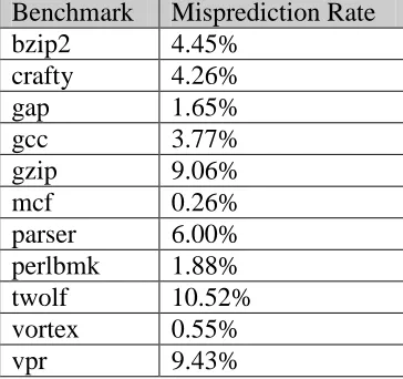
Table 1. Misprediction rates for the large gshare branch predictor used in this section. In the graphs of Figure 3, the 0% point represents performance with these accuracies.

Benchmark Misprediction Rate

bzip2 4.45%

crafty 4.26%

gap 1.65%

gcc 3.77%

gzip 9.06%

mcf 0.26%

parser 6.00% perlbmk 1.88%

twolf 10.52%

vortex 0.55%

vpr 9.43%

(25)

0 1 2 3 4

0% 20% 40% 60% 80% 100%

% of remaining branch mispredictions randomly removed IPC bzip2 gzip twolf 0 1 2 3 4

0% 20% 40% 60% 80% 100%

% of remaining branch mispredictions randomly removed IPC bzip2 gzip twolf 0 1 2 3 4

0% 20% 40% 60% 80% 100%

% of remaining branch mispredictions randomly removed IPC crafty gap gcc perl vortex 0 1 2 3 4

0% 20% 40% 60% 80% 100%

% of remaining branch mispredictions randomly remaining IPC crafty gap gcc perl vortex 0 1 2 3 4

0% 20% 40% 60% 80% 100%

% of remaining branch mispredictions randomly removed IPC mcf 0 1 2 3 4

0% 20% 40% 60% 80% 100%

% of remaining branch mispredictions randomly removed IPC mcf 0 1 2 3 4

0% 20% 40% 60% 80% 100%

% of remaining branch mispredictions randomly removed IPC parser vpr 0 1 2 3 4

0% 20% 40% 60% 80% 100%

% of remaining branch mispredictions randomly removed

IPC

parser vpr

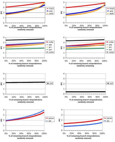
(a) ideal data cache (b) real data cache

(26)

The benchmarks are divided into four groups based on their branch misprediction rates and cache miss rates:

• Bad branch prediction accuracy, good data cache behavior: bzip2, gzip, and twolf.

• Good branch prediction accuracy, good data cache behavior: crafty, gap, gcc, perl,

and vortex.

• Good branch prediction accuracy, bad data cache behavior: mcf.

• Bad branch prediction accuracy, bad data cache behavior: parser and vpr.

In Figure 3, graphs in the left column show results using an ideal data cache (0% data cache miss rate) while graphs in the right column show results with a real data cache.

We are interested in benchmarks from the first and last groups. Benchmarks in the first group have good data cache behavior, which is why their performance does not improve significantly going from the real to the ideal data cache. Removing mispredictions clearly improves the performance of these benchmarks. Achieving perfect branch prediction could double (or almost triple) the performance of these benchmarks. Actually, it not only doubles their performance, but IPC nearly reaches its theoretical maximum of 4 IPC (4-way superscalar). Similarly, benchmarks in the fourth group experience the same behavior, but with either a bigger cache or cache-enhancing techniques such as data prefetching.

(27)

1.2 Understanding the Sources of Branch Mispredictions

1.2.1 Definitions

Today’s best known branch predictors push the envelope of what is possible using global branch or path history as context for making predictions. While this context is basically the same used by precursor predictors since the advent of two-level adaptive branch prediction [55], clever combinations and organizations have yielded nearly perfect branch prediction on some programs and program phases. Yet, results in this dissertation show that branch history alone cannot scale accuracy in other programs beyond 90-95%. In these programs, the leading cause of branch mispredictions are branches that depend directly or indirectly on load instructions.

An example of this type of branches is depicted in Figure 4(a). It shows a static branch at program counter (PC) Z that depends on two static loads at PCs X and Y. At run-time, the static branch translates into many different dynamic branches corresponding to different combinations of load addresses. Two dynamic instances of the branch are shown in Figure 4(b). In the first instance, the two load instructions load from addresses A1 and B1, respectively. In the second instance, the two load instructions load from addresses A2 and B2, respectively. Thus, it is the combination of load addresses that distinguishes one dynamic branch from another. More generally, a dynamic branch is uniquely identified by the combination of its PC and the addresses of loads on which it depends directly or indirectly.

(28)

static load PC X

static load PC Y

static branch PC Z

dynamic load PC X address=A1

dynamic branch PC Z ID = {Z, A1, B1}

dynamic load PC Y address=B1

dynamic load PC X address=A2

dynamic branch PC Z ID = {Z, A2, B2}

dynamic load PC Y address=B2

(a) (b)

Figure 4. (a) A static branch that depends on two static loads. (b) Two dynamic instances of the static branch, one that depends on addresses A1 and B1 and another that depends on addresses A2 and B2.

(29)

sense, the goal of combining PC with global branch history is to forecast which dynamic branch, i.e., which ID, is currently being fetched and to provide a dedicated prediction for it.

(a) (b)

Figure 5. (a) Good scenario: different dynamic branches access different prediction table entries, because different global branch history patterns (P1 versus P2) precede the dynamic branches. (b) Bad scenario: different dynamic branches access the same prediction table entry, because the same global branch history pattern (P1 = P2) precedes the dynamic branches.

On the other hand, if the two dynamic branches are preceded by the same global branch history patterns (P1=P2), they share a prediction table entry. This scenario is depicted in Figure 5(b). One or both of the dynamic branches will be mispredicted if their outcomes differ.

1.2.2 Code Example

This section demonstrates the scenarios explained in Section 1.2.1 using a code example, similar to code in the gzip benchmark. The example is shown in Figure 6. The code has a

while loop that iterates some number of times. Inside the while loop, there is a for loop.

The for loop iterates over an array a that has 16 entries. In the original code in gzip, the size

of the array is much larger. In this example, we are interested in the if branch that tests

(30)

code for the if statement is shown in the small box to the right. A load instruction loads the

contents of a[i], then it is tested with a branch instruction. The branch instruction has a PC

of X. Values of the array elements are shown inside the array. Below each array element is the outcome of the dynamic branch that tests it. The misprediction rate of this branch is 42% for both the gshare [33][32][38][55] and L-TAGE [43] branch predictors, and this would contribute to 20% of the mispredictions in gzip.

The way a gshare branch predictor will try to predict this branch is also shown in Figure 6. If

the predictor is trying to predict the outcome of the dynamic branch testing a[4], it will

hash the PC of the branch (X) with the preceding global branch history which is reflected in the global1_{history register (GHR). To simplify the explanation of this example, we assumed}

that the GHR length is 3-bits.

1

(31)

while(…) {

for(i = 0 ; I < 16 ; i++) {

if ( a[i] > 10)

{ … } else { … } } }

X: BRANCH R5 > 10

a[0] a[1] a[2] a[3] a[4] a[5] a[6] a[7] a[8] a[9] a[10] a[11] a[12] a[13] a[14] a[15] 4 11 15 2 33 7 1 3 52 9 3 8 5 55 8 18

1 0 0 1 0 1 1 1 0 1 1 1 1 0 1 0

Load Value

Branch Outcome

Load Value

1 0 0 1 0 1 1 1 0 1 1 1 1 0 1 0

Branch Outcome

PHT GHR

PC 0 1 0

X LOAD R5, a[i]

+ 0

Figure 6. Code example.

Figure 7 shows the first good scenario where the branch predictor succeeds in predicting the dynamic branch that tests a[4]. The GHR value of 001, used to predict the outcome of

a[4], is unique across the whole array. This will create a dedicated prediction entry for

(32)

Figure 7. Good scenario # 1.

The second good scenario is shown in Figure 8. a[6] is predicted using a GHR value of

101. Similarly, a[10] is predicted using the same GHR value of 101. Both array elements are preceded by the same GHR context which creates a shared prediction entry for both array elements in the PHT. Fortunately, both array elements happen to produce the same branch outcome (taken) which would result in no branch mispredictions.

(33)

The first bad scenario for the same array is shown in Figure 9. Similar to the previous scenario, the predictor tries to predict the branch outcomes of a[6] and a[15] using the same GHR context of 101. Both array elements have the same GHR context which means they will share the same entry in the PHT. Unfortunately, these two elements have different branch outcomes, and will keep overwriting each other in the PHT causing branch mispredictions for either of them, if not for both.

Load Value

1 0 0 1 0 1 1 1 1 0

Branch Outcome

PHT GHR

PC

0 1 1

X

+ ?

a[6] and a[15] have the same GHR context GHR does not distinguish a[6], a[15] Shared prediction entry for a[6], a[15] Unfortunately they have different outcomes

Bad Scenario # 1

1 0 1 1 0 1

shared prediction for a[6], a[15]

Figure 9. Bad scenario # 1.

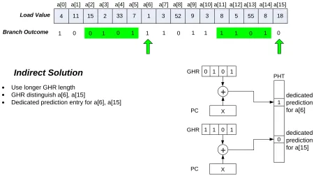
An obvious solution to this problem is to use a longer branch history. Figure 10 shows the

(34)

Load Value

1 0 1 0 1 1 1 0

Branch Outcome

PHT GHR

PC

0 1 1

X

+

1

Use longer GHR length GHR distinguish a[6], a[15]

Dedicated prediction entry for a[6], a[15]

Indirect Solution

1 0 1 1 0 1

dedicated prediction for a[6]

0 1

0

GHR

PC

0 1 1

X

+

0 1

dedicated prediction for a[15]

Figure 10. Indirect solution for bad scenario # 1.

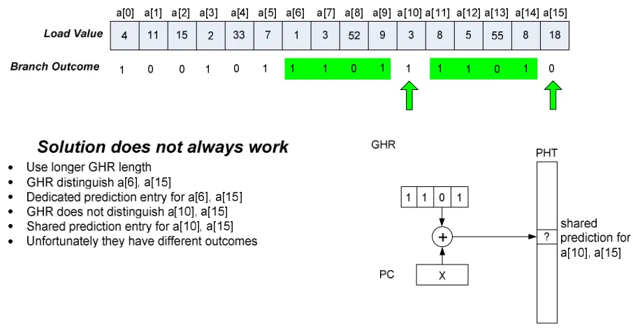
Longer history lengths have been proven to improve the accuracy of the branch predictor [33], simply because it provides more unique context for predicting branches. However, simply increasing history length does not guarantee unique context. Figure 11 shows the same example of a 4-bit GHR but a different pair of elements is highlighted. Notice both

a[10] and a[15] are predicted using the same GHR context of 1101. Unfortunately, the

two elements have different branch outcomes, and this will cause them to negatively interfere in the PHT, causing mispredictions.

(35)

elements will share the same prediction entry. In this way, the branch predictor mirrors the data structure being tested by the branch, since it allocates a dedicated prediction entry per data structure element.

Figure 11. Using longer history does not always work.

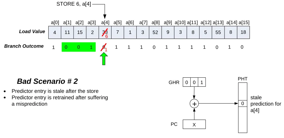
Another bad scenario that could occur is shown in Figure 12. In this case, a[4] is predicted using a 3-bit GHR pattern of 001, which is a unique context throughout the entire array. Once

the branch predictor is trained, it will correctly predict a[4]. However, a store instruction alters the value of a[4] from 33 to 6 which causes the branch outcome of a[4] to flip from

0 to 1. Unfortunately, the branch predictor will have no idea that this happened: when a[4]

(36)

The solution for this problem is to allow store instructions to actively update the branch predictor. This will keep the predictor entries coherent with the data structures it is mirroring.

Load Value

1 0 0 1 0 1 1 1 0 1 1 1 1 0 1 0

Branch Outcome

PHT GHR

PC

0 1 0

X

+ 0

Predictor entry is stale after the store Predictor entry is retrained after suffering a misprediction

Bad Scenario # 2

stale prediction for a[4]

STORE 6, a[4]

6

1

Figure 12. Bad scenario # 2.

1.3 EXACT: Explicit-Dynamic Branch Prediction with Active

Updates

In Chapter 2, we measure the causes of mispredictions using the dynamic-branch framework defined in Section 1.2. We use very large versions of the gselect predictor [33][38][55] and

L-TAGE predictor [43] [41](the latter predictor took first place in the most recent championship branch prediction [57]). The study confirms that the two bad scenarios discussed in Section 1.2.2 are the leading causes of mispredictions in large predictors:

1) Insufficient specialization (bad scenario #1). Often, global branch history, even very

(37)

between two or more dynamic branches. If these dynamic branches have different outcomes, some will be mispredicted because only a single prediction is available to predict all of them.

This problem can be solved by using the branch’s ID to index into the branch predictor. This way, the branch predictor will provide a dedicated entry for each dynamic branch.

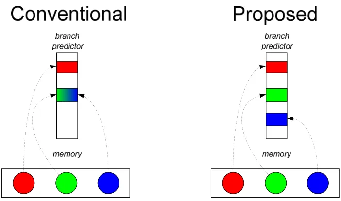
Essentially, a branch predictor should mirror a program’s data objects that are tested by branches. Figure 13 contrasts a conventional history-indexed predictor with the proposed ID-indexed predictor, in terms of their ability to mirror data objects. With the former, multiple data objects in memory might share the same branch predictor entry (the green and blue objects in the figure), which will cause mispredictions if their corresponding branch outcomes are different. The proposed ID-indexed predictor explicitly mirrors data objects, ensuring dedicated branch predictor entries for each data object.

(38)

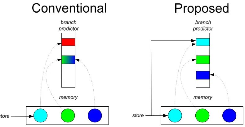
2) Stores (bad scenario #2). A store to an address on which a dynamic branch depends, may cause its outcome to be different the next time it is encountered. In this case, the dynamic branch will be mispredicted because its prediction table entry is stale with respect to the updated data in memory. The entry is only retrained after the misprediction is incurred.

(39)

Figure 14. Second principle: The branch predictor should actively mirror a program’s data objects. (Best if viewed in color.)

We call the proposed predictor EXACT, for “EXplicit dynamic-branch prediction with ACTive updates”. “EX” conveys that dynamic branches are explicitly identified so that they can be provided dedicated predictions and “ACT” conveys that their predictions are actively updated by stores.

We encountered three major implementation challenges while developing the EXACT branch predictor:

1) Using a dynamic branch’s ID to index into the predictor is difficult to do in practice,

because its producer loads are unlikely to have generated their addresses by the time

(40)

2) The most problematic aspect of active updates is converting a store’s address into a

predictor index (or indices) that must be updated. The complexity and storage cost of

address-to-index conversion is potentially prohibitive.

3) Providing a dedicated prediction for each dynamic branch generally requires a large

prediction table. The chief problem with a large prediction table is its long access

time.

(41)

0% 20% 40% 60% 80% 100% 120%

0 200000 400000 600000 800000 1000000 1200000 number of dynamic-branch IDs

cumu

lat

ive % o

f m

is

p

red

ict

ions

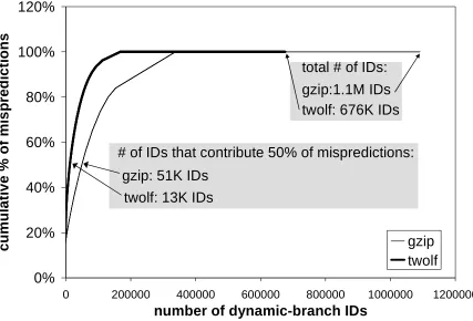
gzip twolf # of IDs that contribute 50% of mispredictions:

gzip: 51K IDs

twolf: 13K IDs

total # of IDs:

twolf: 676K IDs gzip:1.1M IDs

Figure 15. Contributions to mispredictions by different IDs.

In this thesis, we propose two different implementations of EXACT: a hardware-only implementation (EXACT-H) [4] and a combined hardware/software implementation (EXACT-S). EXACT-H and EXACT-S are introduced in Sections 1.3.1 and 1.3.2, respectively.

(42)

index into the predictor cannot be deduced from the load address on which it depends. This leads to a complex and storage-intensive active update unit: a large table is needed to convert store addresses to the predictor indices that must be updated. EXACT-H limits the amount of dedicated storage for its address conversion table by virtualizing it (caching it in the general-purpose memory hierarchy), exploiting the key observation that active updates are tolerant of 100s of cycle of latency.

EXACT-S deals with the first implementation issue by enabling the programmer or compiler to convey key information directly to the fetch unit that it can use to generate branches’ IDs in a timely manner. This yields a number of benefits over EXACT-H. First, EXACT-S is more accurate because it uses branches’ IDs directly rather than prior branches’ IDs. Second, its prediction table is more efficient because global history does not need to be added to the context as in the case of EXACT-H, eliminating unwanted redundancy. Third, with regard to active updates, there is no need for a large table to convert store addresses to predictor indices because of the direct indexing strategy. As a result, active updates are simple and inexpensive in EXACT-S.

(43)

1.3.1 EXACT-H: A Hardware-only Solution

(44)

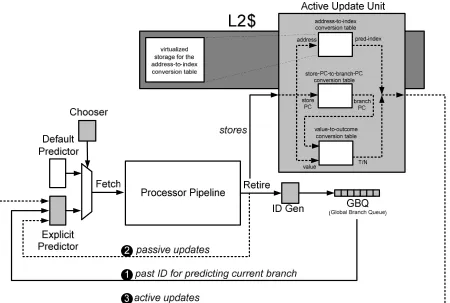
Figure 16. High-level view of EXACT-H.

Indexing Strategy

The ID of a prior retired branch a fixed distance away is a reasonable proxy for the current branch ID because of repetition in the global sequence of dynamic branches. For example, Figure 17(a) shows a sequence of five IDs that repeats. Assuming a distance of 4 is used, ID1

(45)

(a) (b)

(46)

Figure 17(b) shows another example where control-flow affects how to use the proxy ID. Assuming a distance of 4 is used, ID1 is alternately the proxy for both ID5 and ID6. Which

one is to be predicted by a given instance of ID1 depends on the direction of ID4. Therefore,

indexing with only ID1 is unreliable: it would cause ID5 and ID6 to share the same entry in

the predictor (leading to the very problem of lack of specialization that we are trying to solve). To solve this problem, we combine the proxy ID with some recent bits from the global branch history. In the example, ID1 can be combined with the most recent bit of global

branch history to provide two indices, one for ID5 (if the branch outcome of ID4 is not-taken)

and the other for ID6 (if the branch outcome of ID4 is taken).

The chooser of EXACT-H has a mechanism for recognizing the two scenarios in Figure 17. This mechanism is used to learn, for each static branch, whether or not some bits of global history should be included in its index.

Active Update Implementation

Two mechanisms are required for active updates: 1) converting the store address into a predictor index to be updated, and 2) converting the store value into a branch outcome.

(47)

index would be the store address combined with the branch’s PC. To obtain the branch’s PC, EXACT-H learns which static stores affect which static branches by training a small store-PC-to-branch-PC conversion table (Figure 16).

Unfortunately, the dynamic branch’s index is based on a proxy ID. This means its index cannot be determined from the store address directly. Instead, a large address-to-index conversion table is required. The table records, for each address, the explicit predictor’s indices corresponding to dynamic branches that depend on that address.

Converting the store value to a branch outcome is achieved by the value-to-outcome conversion table (Figure 16), which is a reuse table that remembers for each static branch what was the branch’s outcome for different load values. The inputs to this table are the branch’s PC (produced by the store-PC-to-branch-PC conversion) and the store value.

The store-PC-to-branch-PC and value-to-outcome conversion tables are small in size since they record static branch information unlike the address-to-index conversion table that records information about dynamic branches.

(48)

hierarchy (e.g., L2 cache). The advantages include a substantial reduction in dedicated storage, flexible allocation of virtualized active update resources according to application characteristics, and persistence of microarchitectural state.

A potential drawback of virtualization is that it significantly increases the worst-case latency for performing a single active update. Fortunately, latency is not an issue for the active update unit. A key result is that most benchmarks are tolerant of 400+ cycles of latency to perform active updates, due to the long distances between stores and reencounters with branches that they update. This makes the active update unit an ideal candidate for virtualization. Virtualization of the address-to-index conversion table is depicted in Figure 16.

Pipelining the Explicit Predictor

(49)

predictions and post-selecting the finalist at the end of the prediction pipeline when the most recent history bits become available [25][46].

Summary of EXACT-H Results

For equal cost, a hybrid gshare+EXACT-H yields 60%, 30%, and 33% fewer mispredictions than gshare alone, for three misprediction-heavy benchmarks: bzip2, gzip, and twolf, respectively. Similarly L-TAGE+EXACT-H yields 60%, 33%, and 14% fewer mispredictions than L-TAGE alone, for bzip2, gzip, and twolf, respectively.

This thesis explores branch prediction with the view of increasing accuracy when artifacts of limited size, limited history, etc., have already been removed. This is the domain of large branch predictors [25][46], and the domain in which new directions in branch predictor research, such as EXACT, are needed to continue scaling accuracy as conventional history will not.

(50)

comparably to scaling the existing predictor, but without extending the cycle time appreciably. Adding a 4KB explicit predictor cache and 16KB of other overhead (off the critical-path of instruction fetch) removes 33% of mispredictions from a 4KB L-TAGE and 23% of mispredictions from a 8KB L-TAGE. These results are comparable to the accuracy of doubling the L-TAGE size, but without extending cycle time.

1.3.2 EXACT-S: A Combined Hardware/Software Solution

Figure 18 shows a high-level view of EXACT-S. EXACT-S has the same high-level structure as EXACT-H but is simpler.

(51)

Indexing Strategy

The indirect indexing strategy of EXACT-H works reasonably well. However, even with the inclusion of bits from the GHR, there is a significant gap in prediction accuracy between using a distant branch ID and using the current branch ID to index into the explicit predictor. Moreover, indirect indexing is inefficient because it creates redundant entries in the explicit predictor, due to the use of global branch history and multiple proxy IDs leading to the same ID.

EXACT-S exploits software intervention to make the indexing strategy both more accurate and more efficient. In most of the applications that benefit from EXACT, many of the data structures tested by branches are arrays. The fetch unit in EXACT-S features a set of software-managed base registers and offset registers (shown in Figure 18) which enable the fetch unit to calculate the addresses of array elements as the dynamic branches that test them are fetched. This way, a dynamic branch’s ID is known when the branch is fetched, so that the explicit predictor can be indexed directly by the current branch ID.

(52)

of the base and offset registers, hashed with the dynamic branch’s PC to form the ID, as shown in Figure 18.

One approach to enable software to manage the fetch unit is to modify the instruction-set architecture (ISA): (1) add new instructions to write the base and offset registers, and (2) add a bit to conditional branch opcodes to signal whether a static branch should use the explicit predictor or default predictor. There are two drawbacks to this approach. First, it requires changing the ISA which may not be an option. Second, this approach will increase the dynamic instruction count of programs modified to use EXACT-S, reducing the performance gain of EXACT-S.

Therefore, we propose managing the fetch unit with shadow code. Shadow code is appended to the data segment of the program binary. We use the term “shadow” because the programmer or compiler creates a correspondence between selected instructions in the original program and instructions in the shadow code. That is, each shadow-instruction shadows a particular instruction in the original program. Each shadow-instruction is tagged with the PC of the instruction that it shadows. When the instruction is fetched, the shadow-instruction that shadows it is triggered via the PC.

(53)

static branch that tests elements of the array. For example, consider a loop that iterates over an array. The instruction prior to the loop that generates the base address of the array is shadowed by a shadow-instruction in the shadow code called the seed shadow-instruction. The seed shadow-instruction writes the base address into a base register in the fetch unit. An arbitrary instruction prior to the loop is shadowed by a shadow-instruction to initialize an offset register. A convenient instruction within the loop is shadowed by a shadow-instruction that increments the offset register by a certain stride. Finally, a branch within the loop that tests elements of the array is shadowed by a shadow-instruction which signals that the branch should be predicted with the explicit predictor, and which base/offset register pair to use for indexing.

(54)

Note that EXACT-S does not require a chooser (contrast Figure 18 with Figure 16). The shadow code, and the readiness of base registers, controls selection of the explicit predictor or default predictor.

The current implementation of EXACT-S only supports dynamic branches that depend on a single load (single address in the ID), for two reasons. First, the index function does not currently support combining multiple base/offset register pairs, although it is conceivable to do so. Second, and more importantly, supporting dynamic branches that depend on multiple loads would once again require an address-to-index conversion table in the active update unit since the store address is not sufficient to figure out the affected branch ID. That said, it might be practical to do so: while implementing EXACT-H, we have observed that the address-to-index conversion table for multiple-address dynamic branches does not need to be large.

As a final point, while we focused on arrays in the description above, it is possible to target EXACT-S for stable linked-lists as well, as we discuss in Chapter 5. Essentially, they can be treated as virtual arrays.

Active Update Implementation

(55)

update unit simply hashes the store address with the branch PC to determine the index of the dynamic branch that must be updated. Only the store-PC-to-branch-PC and value-to-outcome tables remain. As an alternative to using hardware to train these tables, they can be pre-loaded with information appended to the data segment by the programmer or compiler.

Pipelining the Explicit Predictor

Similar to EXACT-H, the explicit predictor of EXACT-S is scalably pipelinable. If the base register is ready, multiple pipelined accesses to the explicit predictor can be initiated.

Moreover, the indexing strategy of EXACT-S prevents the creation of redundant entries in the explicit predictor: there are no GHR bits in the index and there is no problem of multiple proxy IDs for the same ID. This means the pressure on the explicit predictor will be reduced as compared to EXACT-H, allowing for a smaller explicit predictor for the same effective capacity.

Summary of EXACT-S Results

(56)

(57)

Chapter 2:

Characterizing

Mispredictions

In this chapter, we characterize mispredictions that escape two global history based branch predictors, gselect [33][38][55] and L-TAGE [41][43]. The gselect predictor has a pattern history table (PHT) of 228 entries and the index is formed by concatenating 14 bits of the branch PC with 14 bits of the global branch history register. The L-TAGE predictor is composed of 13 predictor components (a simple bimodal component and 12 other partially tagged components) in addition to a loop predictor. Similar to gselect, the index for each component is formed by concatenating 14 bits of the PC with a component-specific amount of folded global history. A geometric series is used to determine global history lengths for each component ranging from 4 bits to 640 bits. We used the L-TAGE source code provided by the authors [44].

(58)

2.1 Measuring the Ability of History-Based Predictors to Mirror

a Program’s Data Objects

(59)

0% 20% 40% 60% 80% 100% g s e le ct L -T AGE g s e le ct L -T AGE g s e le ct L -T AGE g s e le ct L -T AGE g s e le ct L -T AGE g s e le ct L -T AGE g s e le ct L -T AGE g s e le ct L -T AGE g s e le ct L -T AGE g s e le ct L -T AGE g s e le ct L -T AGE

bzip2 crafty gap gcc gzip mcf parser perlbmk twolf vortex vpr

% d y n a m ic b ra n c h

es match all

value mismatch address mismatch pc mismatch entry miss no address (a) 0% 20% 40% 60% 80% 100% g s e le ct L -T AGE g s e le ct L -T AGE g s e le ct L -T AGE g s e le ct L -T AGE g s e le ct L -T AGE g s e le ct L -T AGE g s e le ct L -T AGE g s e le ct L -T AGE g s e le ct L -T AGE g s e le ct L -T AGE g s e le ct L -T AGE

c o rr . pr e d . as % o f d y n a m ic b ra n c h es match all value mismatch address mismatch pc mismatch entry miss no address (b) 0% 2% 4% 6% 8% 10% 12% g s e le ct L -T AGE g s e le ct L -T AGE g s e le ct L -T AGE g s e le ct L -T AGE g s e le ct L -T AGE g s e le ct L -T AGE g s e le ct L -T AGE g s e le ct L -T AGE g s e le ct L -T AGE g s e le ct L -T AGE g s e le ct L -T AGE

mi s p . a s % of d y n a m ic br a n c h es match all value mismatch address mismatch pc mismatch entry miss no address (c)

(60)

The graphs in Figure 19 show breakdowns of (a) all branches, (b) just correctly predicted branches, as a percentage of all dynamic branches, and (c) just mispredicted branches, as a percentage of all dynamic branches. The percentages in (b) and (c) add up to the percentages in (a). Each bar is broken down into six components. The “no address” component means the dynamic branch either does not depend on any loads or its outcome is not determined solely by loads. From Figure 19(c), the fact that these dynamic branches contribute a relatively small fraction of mispredictions suggests that global history is effective context for specializing predictions for non-load-dependent or non-load-influenced dynamic branches. In Figure 19(a) Gselect and L-TAGE have equal “no address” components because the “no address” component is a property of the program.

The “entry miss” component corresponds to accessing a prediction entry for the first time (cold miss). The “pc mismatch” component corresponds to accessing an entry that was last updated by a different static branch (conflict miss/aliasing). Both are negligible. The “pc mismatch” component is nearly zero, because aliasing among different static branches has been reduced significantly in both predictors (14 PC bits, preserved through concatenation).

(61)

dynamic branches, therefore, the predictor fails to specialize predictions for them. From Figure 19(a), there is an address mismatch in gselect for about 8% (vortex) to 61% (twolf) of all branch predictions and in L-TAGE for about 18% (bzip) to 61% (twolf) of all branch predictions. Mcf has about 100% address mismatches, but it has a very low misprediction rate in the simulated region in any case (its SimPoint [48]).

In relation to the four scenarios described in Chapter 1 (Section 1.2.2), the “address mismatch” component in Figure 19(b) corresponds to good scenario #2, where two dynamic branches have the same global branch history context and the same branch outcome. The “address mismatch” component in Figure 19(c) corresponds to bad scenario #1, where two dynamic branches have the same global branch history context but different branch outcomes.

(62)

2.2 Measuring the Effect of Stores on Modifying Branch

Outcomes

The “value mismatch” component in Figure 19 corresponds to the case where the dynamic branch being predicted is the same as the dynamic branch which last updated the prediction entry (their IDs match), but the values at its load addresses were changed by stores since it last updated the prediction entry. To detect this case, each prediction entry is not only tagged with the ID of the dynamic branch that last updated the entry, but also the values contained at its load addresses at that time.

(63)

(64)

0% 2% 4% 6% 8% 10% 12% gse lect gse lec t+ EX gse lec t+ E X A CT gse lect gse lec t+ EX gse lec t+ E X A CT gse lect gse lec t+ EX gse lec t+ E X A CT gse lect gse lec t+ EX gse lec t+ E X A CT gse lect gse lec t+ EX gse lec t+ E X A CT gse lect gse lec t+ EX gse lec t+ E X A CT gse lect gse lec t+ EX gse lec t+ E X A CT gse lect gse lec t+ EX gse lec t+ E X A CT gse lect gse lec t+ EX gse lec t+ E X A CT gse lect gse lec t+ EX gse lec t+ E X A CT gse lect gse lec t+ EX gse lec t+ E X A CT

mi s p . a s % of d y n a m ic br a n c h es match all value mismatch address mismatch pc mismatch entry miss no address (a) 0% 2% 4% 6% 8% 10% 12% L -T A GE L -TA G E + EX L -T A G E + E X A CT L -T A GE L -TA G E + EX L -T A G E + E X A CT L -T A GE L -TA G E + EX L -T A G E + E X A CT L -T A GE L -TA G E + EX L -T A G E + E X A CT L -T A GE L -TA G E + EX L -T A G E + E X A CT L -T A GE L -TA G E + EX L -T A G E + E X A CT L -T A GE L -TA G E + EX L -T A G E + E X A CT L -T A GE L -TA G E + EX L -T A G E + E X A CT L -T A GE L -TA G E + EX L -T A G E + E X A CT L -T A GE L -TA G E + EX L -T A G E + E X A CT L -T A GE L -TA G E + EX L -T A G E + E X A CT

mi s p . a s % of d y n a m ic br a n c h es match all value mismatch address mismatch pc mismatch entry miss no address (b)

Figure 20. Combining the idealized explicit dynamic-branch predictor with (a) gselect and (b) L-TAGE.

(65)

(66)

to substantially reduce the misprediction rate with respect to gselect and L-TAGE. From Figure 20(b), bzip, crafty, gzip, and twolf, the four benchmarks which experienced the largest increases in “value mismatch” type mispredictions, have many of these mispredictions eliminated by active updates, for a substantial decrease in the overall misprediction rate with respect to L-TAGE.

(67)

Chapter 3:

The Microarchitecture of

EXACT-H

Figure 21 shows the major components of the EXACT-H predictor. A prediction is supplied by either the default predictor (e.g., L-TAGE) or the explicit predictor. The explicit predictor is simply a table of 1-bit predictions. The chooser classifies static branches as more suitable for the default predictor or the explicit predictor. The chooser also singles out static branches that exhibit loop behavior and directs an explicit loop predictor to provide a trip-count to the fetch unit instead of single prediction.

Chooser

Explicit

Predictor

Explicit

Loop

Predictor

Default

Predictor

Active

Update

Unit

ID Generation

Unit

Global Branch Queue

GBQ

ID

trip-count T/NT pred.

Figure 21. Major components of EXACT-H.

(68)

pushed onto the global branch queue (GBQ). The GBQ is used for indexing the explicit predictor and explicit loop predictor.

Sections 3.1 through 3.4 explain ID generation, the GBQ, indexing the explicit predictor, and pipelining the explicit predictor. The explicit loop predictor, chooser, and active update unit are explained in Sections 3.5 through 3.7.

3.1 ID Generation Unit

A non-functional architectural register file (ARF) propagates addresses of loads to branches that depend on them directly or indirectly. In this work, each logical register in the ARF holds up to four load addresses. Loads write their addresses into their destination registers when they retire from the load queue. ALU instructions propagate addresses from their source registers to their destination registers when they retire from the reorder buffer. Branch instructions obtain their load addresses from their source registers when they retire from the reorder buffer.

(69)

register in the ARF. In summary, load addresses are propagated to branches through both registers and the stack.

Figure 22. Hash function for generating a dynamic branch’s ID.

A dynamic branch forms its ID by hashing its PC and load addresses together, as follows. The first address is XORed with the second address shifted left by one bit, the third address shifted left by two bits, and so on, for as many load addresses as there are. The result is then ANDed with a mask to extract the low N bits, for an explicit predictor that has 2N entries. The upper 8 bits of the result is XORed with the lower 8 bits of the PC. Figure 22 describes the hash function in C code, for N=20.

3.2 Global Branch Queue

The GBQ contains IDs of recently retired dynamic branches. When a dynamic branch retires, the ID generation unit pushes its ID onto the GBQ, displacing the oldest ID in the GBQ. GBQ length is discussed in the next section.

3.3 Indexing the Explicit Predictor

We cannot use the ID of a dynamic branch to index the explicit predictor for two reasons. First, typically, its producer loads have not generated their addresses by the time it is fetched. Second, even if addresses were available in time to predict the branch, assembling and

hash = 0;

for (i = 0; i < num_addresses; i++) hash = hash ^ (address[i] << i);

hash = hash & 0xFFFFF; // this mask corresponds to N=20

(70)

associating them with the branch currently being fetched is challenging, whereas the ID generation unit does this straightforwardly when the branch itself retires.

Instead, the index for a branch is based on the ID of a prior retired branch some fixed distance away. This distance determines the length of the GBQ. The approach is illustrated in Figure 23 for three scenarios and a distance of 20. The three scenarios differ in how many unretired branches are currently in the processor pipeline, affecting which branch in the GBQ is used to predict the new branch. The third scenario shows what happens when the distance between the new branch and the youngest retired branch in the GBQ is greater than the fixed distance, 20. The problem is that the new branch needs the ID of a branch which has not yet retired. It cannot form an index into the explicit predictor and must use the default predictor instead.

KEY

retired branch (GBQ entry)

unretired branch

new branch

Branches in GBQ Branches in Processor Pipeline

?? Scenario #1

Scenario #2

Scenario #3

(71)

This indexing strategy is tantamount to predicting the ID of the current branch from the ID of a distant prior branch. A given ID may lead to any of a number of IDs downstream from it, depending on intervening control-flow (among other things). This is corroborated by our studies which show that hashing the ID of the distant prior branch with global branch history is essential for more closely approximating using the ID of the current branch. We have observed a few exceptions to this general rule. In these exceptional cases, including global branch history may be detrimental because it creates redundant entries in the explicit predictor which has two negative effects: thrashing the predictor and needlessly increases training time. We concluded that global branch history should be used for some branches and not others. To this end, the chooser – in addition to selecting among the default predictor, explicit predictor, and explicit loop predictor – identifies branches whose indices into the explicit predictor should not include global branch history.

When global branch history is included in the index, it is hashed into the low bits of the ID of the distant prior branch. Figure 24 describes the index function in C code, for a distance of 20 and 6 branch history bits.

Figure 24. Example index function, described in C code.

Figure 25 shows the effect of distance, for two cases: (a) the prior branch whose ID is used for the index is assumed to be retired regardless of distance (i.e., never suffer scenario #3),

// 1. ID_20 is the ID of the branch that is 20 branches away // 2. BHR is the global branch history register

// 3. use_history is from the chooser

(72)

and (b) whether or not the prior branch is retired is determined through cycle-level processor simulation (may suffer scenario #3).

0% 2% 4% 6% 8% 10% 12%

0 2 4 6 8 10 12 14 16 18 20 22 24 26 28 30

distance

m

is

pr

e

d

ic

ti

on

r

at

e

%

bzip2 crafty gzip twolf

(a)

0% 2% 4% 6% 8% 10% 12%

0 2 4 6 8 10 12 14 16 18 20 22 24 26 28 30

distance

m

is

pr

e

d

ic

ti

on

r

a

te

%

bzip2 crafty gzip twolf

(b)

Figure 25. Effect of distance. (a) Prior branch is always retired. (b) Retired status based on processor simulation.

(73)

almost exclusively. Case (a) shows increasing misprediction rate with distance, with gzip and twolf showing large jumps between distance 0 and 1. This transition is effectively the gap between ideal and real index prediction. Subsequently, misprediction rate increases gradually with increasing distance. Case (b) shows decreasing misprediction rate with distance since increasing distance increases the number of branches predicted by the explicit predictor. Cases (a) and (b) converge in the low to mid 20s for gzip and twolf.

The rationale behind using the branch ID at a fixed distance as the index, is repetition in the dynamic branch stream. Changes in intervening control-flow may cause different streams. Using recent global branch history in the index accounts for this.

3.4 Pipelining the Explicit Predictor

(74)

+ + +

+ +

+ GBQ

ID1 + BHR

ID2

+ BHR

ID3

+ BHR

CYCLE 1 CYCLE 2 CYCLE 3 CYCLE 4 CYCLE 5 CYCLE 6 CYCLE 7

Figure 26. Pipelining the explicit predictor. Diagram shows three consecutive accesses to a three-cycle-latency predictor.

(75)

bits are generated at the end of the prediction pipeline (by which time the preceding pending accesses have produced their predictions), which control the MUX.

3.5 Explicit Loop Predictor

Some loops have trip-counts that depend on one or more loads preceding the loop. An example of such a loop from twolf is shown in Figure 27 and explained in the figure caption. Applying the same static vs. dynamic framework defined in Chapter 1, Section 1.2.1, we say that a static trip-count translates into multiple dynamic trip-counts at run-time. Like a dynamic branch, a dynamic trip-count has an identity (ID) as a whole: the PC of the loop branch combined with the addresses of loads that the dynamic trip-count depends on. Different dynamic trip-counts are distinguished by their IDs. The role of the explicit loop predictor is to provide specialized trip-count predictions to different dynamic trip-counts, analogous to the role of the explicit predictor for dynamic branches.

Figure 27. Example for-loop in the sub_penal() function in twolf. The trip-count of the loop branch is dynamic and transitively depends on three heap loads in the caller function ucxx1(). The transitive dependence is shown with boldface type.

ucxx1(...) { ...

int axcenter, aleft, aright, a1LoBin, a1HiBin; ...

axcenter = acellptr->cxcenter ; // heap load

aleft = atileptr->left ; // heap load

aright = atileptr->right ; // heap load ...

a1LoBin = SetBin( startxa1 = axcenter + aleft ); // SetBin() is a simple macro

a1HiBin = SetBin( endxa1 = axcenter + aright ); ...

sub_penal( ... , a1LoBin , a1HiBin ); ...

}

sub_penal( ... , int LoBin , int HiBin ) { ...

for ( bin = LoBin ; bin <= HiBin ; bin++ ) { // example for-loop ...

(76)

The explicit loop predictor is accessed using the same index as the explicit predictor (Section 3.3). The explicit loop predictor is managed as a set-associative cache, however, so it can have fewer entries yet still use the full-length indices. The low bits of the index select a set. Entries within the set are tagged with the remaining high bits of the index. An entry is shown in Figure 28.

tag

trip-count

valid bit

LRU bits

cache management payload

Figure 28. A single entry in the explicit loop predictor.

(77)

3.6 Chooser

The chooser has three jobs: 1) identify branches that are best predicted by the default predictor (§3.6.1), 2) identify branches that exhibit dynamic trip-counts, hence, are best predicted by the explicit loop predictor if it hits or the default predictor otherwise (§3.6.2), and 3) identify branches that do not need global branch history included in their indices (§3.6.3).

The chooser is PC-indexed and is not tagged. Thus, classification is on a per-static-branch basis. This is not only efficient in terms of storage but it also enables rapid classification since all dynamic instances of a static branch train its entry.

3.6.1 Choosing the Default Predictor

(78)

predictors are incorrect and correct, respectively; and unchanged when both predictors are correct or incorrect. If the counter saturates, the sticky bit is set. A sticky bit of 1 signifies that the default predictor should be used for all dynamic instances of the static branch. Crucially, dynamic instances of this static branch no longer participate in training the explicit predictor or active update unit, dedicating these important resources to more suitable branches.

Certain load-dependent branches are best left for the default predictor for two reasons. First, the indexing strategy may not be accurate for these branches. Recall that this strategy is tantamount to inferring the current branch’s ID from a previous branch’s ID, a form of address prediction. This may be inaccurate for some branches and they should be weeded out. Second, there may be thrashing in the explicit predictor: explicitly mirroring memory is a worthy cause but requires sufficient predictor capacity, and off-loading some branches to the default predictor may be necessary.

EXACT: Explicit Dynamic-Branch Prediction with Active Updates.

Abstract

Dedication

Biography

Acknowledgments

Table of Contents

List of Figures

List of Tables

Chapter 1:

Introduction

1.1

Background

1.1.1

Superscalar Processors and ILP

1.1.2

Branch Instructions and Branch Prediction

1.1.3

Quantifying the Effect of Branch Mispredictions on Performance

1.2

Understanding the Sources of Branch Mispredictions

1.2.1

Definitions

1.2.2

Code Example

1.3