FIR Digital Filter and Neural Network Design using Harmony Search Algorithm

(1)

University of Windsor University of Windsor

Scholarship at UWindsor

Electronic Theses and Dissertations Theses, Dissertations, and Major Papers

9-6-2018

FIR Digital Filter and Neural Network Design using Harmony

Search Algorithm

ABIRA PAUL

University of Windsor

Follow this and additional works at: https://scholar.uwindsor.ca/etd

Recommended Citation Recommended Citation

PAUL, ABIRA, "FIR Digital Filter and Neural Network Design using Harmony Search Algorithm" (2018). Electronic Theses and Dissertations. 7556.

https://scholar.uwindsor.ca/etd/7556

This online database contains the full-text of PhD dissertations and Masters’ theses of University of Windsor students from 1954 forward. These documents are made available for personal study and research purposes only, in accordance with the Canadian Copyright Act and the Creative Commons license—CC BY-NC-ND (Attribution, Non-Commercial, No Derivative Works). Under this license, works must always be attributed to the copyright holder (original author), cannot be used for any commercial purposes, and may not be altered. Any other use would require the permission of the copyright holder. Students may inquire about withdrawing their dissertation and/or thesis from this database. For additional inquiries, please contact the repository administrator via email

(2)

FIR Digital Filter and Neural Network design using Harmony Search

Algorithm

By

Abira Paul

A Thesis

Submitted to the Faculty of Graduate Studies

through the Department of Electrical and Computer Engineering

in Partial Fulfillment of the Requirements for the Degree

of Master of Applied Science at the University of Windsor

Windsor, Ontario, Canada

2018

(3)

FIR Digital Filter and Neural Network design using Harmony Search

Algorithm

by

Abira Paul

APPROVED BY:

______________________________________________ F. Baki

Odette School of Business

______________________________________________ H. Wu

Department of Electrical and Computer Engineering

______________________________________________ H. K. Kwan, Advisor

Department of Electrical and Computer Engineering

(4)

iii

DECLARATION OF ORIGINALITY

I hereby certify that I am the sole author of this thesis and that no part of this thesis has been

published or submitted for publication.

I certify that, to the best of my knowledge, my thesis does not infringe upon anyone’s copyright

nor violate any proprietary rights and that any ideas, techniques, quotations, or any other

material from the work of other people included in my thesis, published or otherwise, are fully

acknowledged in accordance with the standard referencing practices. Furthermore, to the extent

that I have included copyrighted material that surpasses the bounds of fair dealing within the

meaning of the Canada Copyright Act, I certify that I have obtained a written permission from

the copyright owner(s) to include such material(s) in my thesis and have included copies of

such copyright clearances to my appendix.

I declare that this is a true copy of my thesis, including any final revisions, as approved by my

thesis committee and the Graduate Studies office and that this thesis has not been submitted for

(5)

iv

ABSTRACT

Harmony Search (HS) is an emerging metaheuristic algorithm inspired by the improvisation

process of jazz musicians. In the HS algorithm, each musician (= decision variable) plays (=

generates) a note (= a value) for finding the best harmony (= global optimum) all together. This

algorithm has been employed to cope with numerous tasks in the past decade. In this thesis, HS

algorithm has been applied to design digital filters of orders 24 and 48 as well as the parameters

of neural network problems. Both multiobjective and single objective optimization techniques

were applied to design FIR digital filters. 2-dimensional digital filters can be used for image

processing and neural networks can be used for medical image diagnosis. Digital filter design

using Harmony Search Algorithm can achieve results close to Parks McClellan Algorithm

which shows that the algorithm is capable of solving complex engineering problems. Harmony

Search is able to optimize the parameter values of feedforward network problems and fuzzy

inference neural networks. The performance of a designed neural network was tested by

introducing various noise levels at the testing inputs and the output of the neural networks with

noise was compared to that without noise. It was observed that, even if noise is being introduced

to the testing input there was not much difference in the output. Design results were obtained

(6)

v

DEDICATION

Dedicated to,

(7)

vi

ACKNOWLEDGEMENTS

I would like to thank my supervisor Dr. H.K. Kwan for introducing me the methodologies of

designing digital filters, neural networks, and fuzzy neural networks using Harmony Search

algorithm and suggesting it as the project of my thesis. His guidance and support throughout

my M.App.Sc helped me to achieve successes. I would also like to thank my committee

members for providing their valuable inputs. A special thanks to my fellow students Rija Raju,

Jiajun Liang and Miao Zhang for discussions.

I would like to pay my special regards to the University of Windsor for providing an excellent

environment for carrying out my study. Last but not the least I would extend my thanks to my

(8)

vii

TABLE OF CONTENTS

DECLARATION OF ORIGINALITY ... iii

ABSTRACT ... iv

DEDICATION ... v

ACKNOWLEDGEMENTS ... vi

LIST OF TABLES ... ix

LIST OF FIGURES ... x

LIST OF ABBREVIATIONS/SYMBOLS ... xi

Introduction ... 1

1.1 Why Digital Filters? ... 1

1.2 Types of Filters ... 2

1.2.1 Based on frequency response ... 2

1.2.2 Based on impulse response ... 2

1.3 FIR Filters ... 2

1.3.1 Linear phase FIR filters ... 4

1.3.2 Equiripple design of linear phase FIR filters ... 6

1.3.3 Constrained equiripple FIR filters ... 9

1.3.4 Difference between equiripple design and least squared FIR filter design ... 9

1.3.5 Why are FIR filters preferred over IIR filters? ... 10

1.3.6 General phase FIR filters ... 10

1.4 Quantization of coefficients ... 12

1.4.1 Initial Coefficient Values for Populations ... 13

1.5 Filter Design Problems ... 13

1.5.1 Deterministic algorithms ... 16

1.5.2 Heuristic algorithms ... 16

1.5.3 Metaheuristic algorithms ... 17

1.5.4 Evolutionary algorithms ... 18

1.6 Neural Networks... 20

1.7 Contributions ... 20

(9)

viii

... 22

2.1 Survey of Harmony Search Applications ... 23

2.2 What is Harmony Search Algorithm? ... 24

2.3 Design of Harmony Search Algorithm ... 24

2.4 Improvements in Harmony Search Algorithm ... 26

2.5 Why is Harmony Search successful? ... 27

2.6 Introduction to Neural Networks ... 28

2.7 Why Neural Networks? ... 29

2.8 Types of Neural Networks ... 30

2.8.1 Feedforward neural networks ... 30

2.8.2 Fuzzy neural networks ... 30

... 32

3.1 FIR Filter Design ... 32

3.2 Neural Network Design ... 33

3.2.1 Design using XOR neural network ... 33

3.2.2 Design using feedforward neural networks ... 34

3.2.3 XOR design using min-sum fuzzy inference network ... 37

... 40

4.1 Results ... 40

4.1.1 Linear phase order 24 FIR filter design obtained Using HS ... 40

4.1.2 Linear Phase Results compared with FIRPM for order 24 ... 44

4.1.3 Linear Phase order 48 results obtained Using HS ... 47

4.1.4 Linear Phase Results compared with FIRPM for order 48 ... 51

4.1.5 General FIR Results obtained Using HS for Order 24 ... 54

4.1.6 Design using XOR neural network ... 57

4.1.7 Digit recognition using feedforward neural network ... 59

4.1.8 XOR design using min-sum fuzzy inference network ... 65

... 67

REFERENCES ... 70

(10)

ix

LIST OF TABLES

Table 1.1 Symmetric filters ... 4

Table 1.2 Comparison between FIR and IIR filters ... 10

Table 1.3 Comparing the performance of the HSA algorithm with other algorithms using Test functions ... 19

Table 3.1 Training data sets: Nine training Samples for Fuzzy Exclusive XOR Problem ... 38

Table 4.1 Coefficients of order 24 Type I Lowpass LP-FIR filter by HS ... 41

Table 4.2 Coefficients of order 24 Type1 Bandpass LP-FIR filter by HS ... 42

Table 4.3 Coefficients of order 24 Type1 Highpass LP-FIR filter by HS ... 43

Table 4.4 Coefficients of order 24 Type1 Bandstop LP-FIR filter by HS ... 44

Table 4.5 Order 24 FIR type 1 filter design results comparison (PM: Parks McClellan; HS: Harmony Search) ... 46

Table 4.6 Coefficients of order 48 Type1 Lowpass LP-FIR filter by HS ... 48

Table 4.7 Coefficients of order 48 Type1 Bandpass LP-FIR filter by HS ... 50

Table 4.8 Order 48 FIR type 1 filter design results comparison (PM: Parks McClellan; HS: Harmony Search) ... 52

Table 4.9 Lowpass, Highpass, Bandpass, and Bandstop digital filter cutoff frequencies ... 52

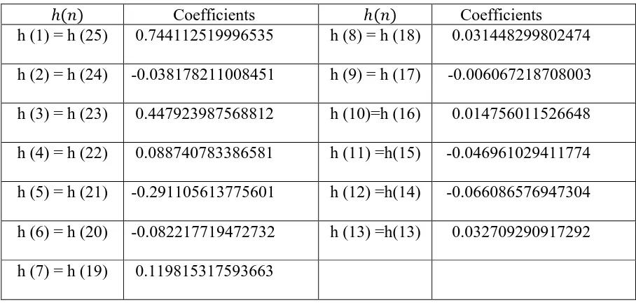
Table 4.10 Linear Phase FIR Filter Coefficients (Order 24) ... 52

Table 4.11 Linear Phase FIR Filter Coefficients (Order 48) ... 53

Table 4.12 Coefficients of order 24 type1 Lowpass LP-GFIR filter by HS ... 55

Table 4.13 Coefficients of order 24 type1 Bandpass LP-GFIR filter by HS ... 56

Table 4.14 Order 24 General FIR Type 1 filter design results using HS ... 56

Table 4.15 2-input one output Neural network design parameters ... 57

Table 4.16 2-input one output Neural network design ... 57

Table 4.17 Computational results of the feedforward neural network design for ten hidden neurons (without noise) ... 59

Table 4.18 Comparison of results with the ideal output and the Mean Square errors for each of the four output neurons ... 59

Table 4.19 Computational results of the feedforward neural network design for ten hidden neurons (40% noise) ... 60

Table 4.20 Comparison of results with the ideal output and the Mean Square errors for each of the four output neurons ... 60

Table 4.21 Computational results of the feedforward neural network design for eight hidden neurons (without noise) ... 62

Table 4.22 Computational results of the feedforward neural network design for eight hidden neurons (without noise) ... 62

Table 4.23 Computational results of the feedforward neural network design for eight hidden neurons (40% noise) ... 63

Table 4.24 Computational results of the feedforward neural network design for eight hidden neurons (40% noise) ... 63

Table 4.25 Computational results of the min sum fuzzy neural network design (without noise) ... 65

(11)

x

LIST OF FIGURES

Figure 1.1 Types of filters based on frequency response ... 2

Figure 1.2 Block diagram of FIR filter ... 3

Figure 1.3 FIR in direct form ... 3

Figure 1.4 FIR filter in transposed direct form ... 3

Figure 1.5 Type I Linear phase FIR coefficients ... 5

Figure 1.6 Phase response of linear phase FIR filter ... 6

Figure 1.7 Lowpass filter design specifications (Kwan[18], 2016, Pg 18) ... 8

Figure 1.8 Design of equiripple FIR filters using FIRPM ... 9

Figure 3.1 Neural network design for two input XOR problem [18] ... 33

Figure 3.2 Training pattern pairs (Kwan[22], 1992, pg 2) ... 36

Figure 4.1 Order 24 linear phase lowpass FIR digital filter using HS ... 40

Figure 4.2 Order 24 linear phase bandpass FIR digital filter using HS ... 41

Figure 4.3 Order 24 linear phase highpass FIR digital filter using HS ... 42

Figure 4.4 Order 24 linear phase bandstop FIR digital filter using HS ... 43

Figure 4.5 Lowpass FIR filter comparing HS and FIRPM ... 44

Figure 4.6 Bandpass FIR filter comparing HS and FIRPM ... 45

Figure 4.7 Highpass FIR filter comparing HS and FIRPM ... 45

Figure 4.8 Bandstop FIR filter comparing HS and FIRPM ... 46

Figure 4.9 Order 48 linear phase lowpass FIR digital filter using HS ... 47

Figure 4.10 Order 48 linear phase bandpass FIR digital filter using HS ... 49

Figure 4.11 Lowpass FIR Filter comparing HS and FIRPM ... 51

Figure 4.12 Bandpass FIR Filter comparing HS and FIRPM... 51

Figure 4.13 Order 24 general phase lowpass FIR digital filter using HS ... 54

Figure 4.14 Order 24 general phase bandpass FIR digital filter using HS ... 54

Figure 4.15 Two dimensional view of XOR neural network ... 58

Figure 4.16 Plot of the 1054 weight vectors for ten hidden neurons... 61

Figure 4.17 Plot of the 844 weight vectors for eight hidden neurons ... 64

(12)

xi

LIST OF ABBREVIATIONS/SYMBOLS

HS Harmony Search

HSA Harmony Search Algorithm

Fig Figure

𝐻(𝑤) Frequency response of the Filter

ℎ𝑛 𝑛𝑡ℎ Filter coefficient

PM Parks McClellan

Gd Group delay of the passband

𝛿 Passband ripple

𝛿𝑝 Specified Passband ripple

𝛿_𝑠 Specified Stopband ripple

𝑊_𝑠(𝑤𝑖) Weighing function

𝑤𝑝 Passband cut off frequency

(13)

1

Introduction

1.1 Why Digital Filters?

What are Digital Filters?

In signal processing, a digital filter is a system that performs mathematical operations on sampled, discrete-time signal to reduce or enhance certain aspects of the signal as it may be necessary.

The applications of digital filters are widespread some of which includes the following:

• Communication Systems

• Image processing and enhancement

• Instrumentation

• Processing of biological signals

The digital filters are used in communication systems because of their ability to minimize error

probability and producing quality signal. In image processing, the digital filters are used mainly

to suppress either the high frequencies in the image, or the low frequencies i.e. enhancing or

detecting the edges in the image. Filters alter the frequency spectrum of the input signal and

thus are used in instrumentation. The digital filters have also been used for biomedical signal

processing.

Before proceeding with the details and moving onto further depth, I will like to mention that in

this thesis I have tried to show how to solve complex problems such as Digital Filters and

Neural network designs in less time in an efficient manner as an alternative to other

metaheuristic algorithms using a particular metaheuristic algorithm called Harmony Search

Algorithm. This metaheuristic algorithm was initially used with Particle Swarm Optimization

for the design of Infinite Response Filters for improved performance and also for many

industrial applications discussed in the Chapter 2 in Section 2.2. However designing of FIR

digital Filters and feedforward neural networks is a new concept which have not been addressed

(14)

2

1.2 Types of Filters

1.2.1 Based on frequency response

Based on the frequency response, the filters can be categorized into four common types as

shown in Figure 1-1.

Figure 1.1 Types of filters based on frequency response

1.2.2 Based on impulse response

Based on the impulse response, there are two categories of digital filters; namely finite impulse

response filters(FIR) and infinite impulse response filters(IIR). The significant difference

between FIR and IIR filter is that in case of FIR filter, the output decays to 0 in a finite amount

of time, whereas in case of IIR filter the output takes an infinite amount of time to decay to 0.

1.3 FIR Filters

FIR Filters are digital filters with the finite impulse response. They are also known as

(15)

3

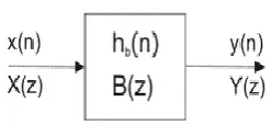
Figure 1.2 Block diagram of FIR filter

Figure 1.3 FIR in direct form

T=decay

ℎ0, ℎ1… … ℎ𝑛−1 = Filter coefficients

𝑥[𝑘], 𝑥[𝑘 − 1], … … 𝑥[𝑘 − 𝑁 + 1]=Input and a delayed version of the input

𝑦[𝑘] = Output of the filter

The output of the filter can be written in the following equation form:

𝑦[𝑘] = ℎ0𝑥[𝑘] + ℎ1𝑥[𝑘 − 1] + ⋯ + ℎ𝑛−1𝑥[𝑘 − 𝑁 + 1] (1. 1)

(16)

4 1.3.1 Linear phase FIR filters

Depending on the order of the filters and the symmetry of the filter coefficients, the linear phase filters can be of four types [25] as shown in the following Table:

Table 1.1 Symmetric filters

Order Symmetry 𝑯(𝒘) 𝒂𝒕 𝒘 = 𝟎 _{𝑯(𝒘)𝒂𝒕 𝒘 = 𝝅 𝑻}⁄

Type I Even Even Any Any

Type II Odd Even Any 0

Type III Even Odd 0 Any

Type IV Odd Odd 0 0

If ℎ₀, ℎ₁… … … ℎ_𝑁−1 are the filter coefficients, where 𝑁 is the length of the filter, then the

following relations hold for the coefficients of the different kinds of filters.

Type I: ℎ𝑘 = ℎ𝑁−𝑘+1, 𝑁 is odd

Type II:ℎ𝑘 = ℎ𝑁−𝑘+1, 𝑁 is even

Type III:ℎ_𝑘 = −ℎ_{𝑁−𝑘+1}, 𝑁 is even

Type IV:ℎ_𝑘 = −ℎ_{𝑁−𝑘+1}, 𝑁 is odd

The amplitude response of the four types of filters can be expressed in the following equations:

Type I:

𝐻(𝑤) = ℎ(𝑀) + 2 ∑ ℎ𝑛cos((𝑀 − 𝑛)𝑤) 𝑀−1

𝑛=0

(1.2)

Type II:

𝐻(𝑤) = 2 ∑ ℎ𝑛cos((𝑀 − 𝑛)𝑤) 𝑁 2 ⁄ −1 𝑛=0 (1.3) Type III

𝐻(𝑤) = 2 ∑ ℎ𝑛sin((𝑀 − 𝑛)𝑤) 𝑀−1

𝑛=0

(1.4)

(17)

5

𝐻(𝑤) = 2 ∑ ℎ𝑛 𝑁

2 ⁄ −1

𝑛=0

cos((𝑀 − 𝑛)𝑤) (1.5)

Where, 𝑀 = (𝑁 − 1) 2⁄

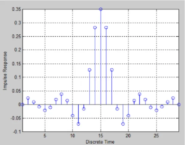
In the following figure, the filter coefficient values of Type I Linear phase filter can be shown:

Figure 1.5 Type I Linear phase FIR coefficients

The coefficients are symmetric around the central coefficient. The phase response of the

(18)

6

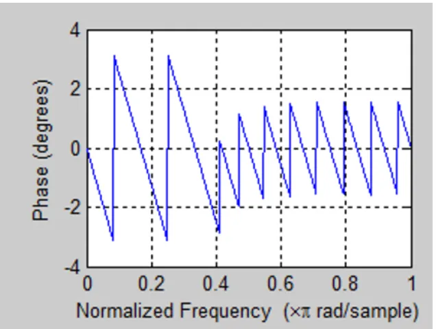
Figure 1.6 Phase response of linear phase FIR filter

We can see that the phase response of the filter varies linearly. The discontinuities are mainly

due to two reasons:

1)2𝜋 + 𝜃 = 𝜃 resulting the phase being confined from −𝜋 𝑡𝑜 𝜋

2) The sign reversal of the frequency response.

1.3.2 Equiripple design of linear phase FIR filters

The finite length Impulse response of Filter (FIR) has the exact linear phase. FIR filters can be

realized by the causal system because after time delaying any non-causal sequence can be

causal.

The transfer function of the Type I Filter is given as:

𝐻(𝑐, 𝑤) = 𝑒−𝑗(𝑀−12 )𝑤𝑇

{

ℎ (𝑀 − 1

2 ) + ∑ 2ℎ(𝑛)𝑐𝑜𝑠 [( 𝑀 − 1

2 − 𝑛) 𝑤𝑇]

𝑀−3 2

𝑛=0

}

(1.6)

𝐻(𝑐, 𝑤) = 𝑒−𝑗(𝑀−12 )𝑤𝑇_{𝐴(𝑐, 𝑤) (1.7)}

(19)

7

Where,

𝐴(𝑐, 𝑤) = 𝒄𝑻𝑐𝑜𝑠 𝑤 (1.8)

And,

cos 𝑤 = [1 𝑐𝑜𝑠(𝑤𝑇) 𝑐𝑜𝑠(2𝑤𝑇) … . . 𝑐𝑜𝑠 (𝑀 − 1 2 𝑤𝑇)]

𝑇

(1.9)

The coefficient vector 𝑐𝑇 is optimized initially using some random values and then the

objective function value is reduced at every iteration by following the structure of the algorithm

which has been reduced by minimizing the value of the error at every iteration. The minimax

error approximation method is used to calculate the error. It calculates the difference in error

between the frequency response of the passband and stopband. An ideal filter has a magnitude

of 1 and 0 in the passbands and stopband. The expression of the minimax function has been

shown below: 𝑒𝑝(𝑐) = [∑ 𝑊𝑝(𝑤𝑖) 𝑙_𝑝 𝑖=1 ||𝐴(𝑐, 𝑤𝑖)| − 𝐴𝑑(𝑤𝑖)| 2𝑝 ] 1 2𝑝 ⁄ (1.10)

𝑓𝑜𝑟 𝑊𝑝(𝑤𝑖) ≥ 0; 0 ≤ 𝑤𝑖 ≤ 𝑤𝑝

𝑒𝑠(𝑐) = [∑ 𝑊𝑠 𝑙_𝑠

𝑖=1

(𝑤_𝑖)||𝐴(𝑐, 𝑤_𝑖)| − 𝐴_𝑑(𝑤_𝑖)|2𝑝]

1 2𝑝 ⁄

(1.11)

𝑓𝑜𝑟 𝑊𝑠(𝑤𝑖) ≥ 0; 𝑤𝑠≤ 𝑤𝑖 ≤ 𝜋

Where 𝑒_𝑝(𝑐) and 𝑒_𝑠(𝑐) are the error values in the passband and stopband respectively. 𝐴(𝑐, 𝑤_𝑖)

is the magnitude response of the obtained filter and 𝐴_𝑑(𝑤_𝑖) is the magnitude response of the

ideal filter and i is the number of samples to calculate the error. The minimax optimization

problem is to search for the optimal coefficient vector 𝒄that minimizes the objective function

𝒆(𝒄):

min

𝒄 𝒆(𝒄) (1.12)

𝑊𝑠(𝑤𝑖) represents the weighing function which is given by:

𝑊𝑠(𝑤𝑖) = {1 𝑝𝑎𝑠𝑠𝑏𝑎𝑛𝑑 𝑎𝑛𝑑 𝑠𝑡𝑜𝑝𝑏𝑎𝑛𝑑_{0 𝑒𝑙𝑠𝑒𝑤ℎ𝑒𝑟𝑒} (1.13)

The weighing scores usually differ with the error values; so, if the errors of the passband and

(20)

8

The interval 0 − 𝑤_𝑝 is the passband and 𝑤_𝑐 − 1 is the stopband of the filter. The response

usually varies from 1 − 𝛿_𝑝 to 1 + 𝛿_𝑝 in the passband and in the stopband, it varies from −𝛿_𝑠 to

𝛿_𝑠 . The transition region which ranges from 𝑤_𝑝 to 𝑤_𝑠 can accept any value.𝛿_𝑝 denotes the

passband ripple whereas 𝛿𝑠 denotes the stopband ripple. The diagrammatic representation is

shown below:

Figure 1.7 Lowpass filter design specifications [25]

The above design problem can be formulated as a linear problem shown below in the following

equations:

Minimize 𝛿

Such that: 1 − 𝛿 ≤ 𝐻(𝑤) ≤ 1 + 𝛿, 𝑓𝑜𝑟 𝜔 ∈ [0, 𝜔𝑝] (1.14)

− (𝛿𝑠𝛿) 𝛿⁄ 𝑝≤ 𝐻(𝑤)≤ (𝛿𝑠𝛿) 𝛿⁄ 𝑝, 𝑓𝑜𝑟 𝜔 ∈ [𝑤𝑠, 1]

Where 𝐻(𝑤) is the frequency response of the filter and is given by:

𝐻(𝑤) = ∑ ℎ(𝑛)𝑇𝑟𝑖𝑔(𝑤, 𝑛)

⌈𝑁−1⌉ 2

𝑛=0

(1.15)

Where 𝑇𝑟𝑖𝑔 is the trigonometric function depending on the type of the filter and whether the

(21)

9 1.3.3 Constrained equiripple FIR filters

The design of such filters requires constrained equiripple approximation of an approximate

function. The design is as shown below:

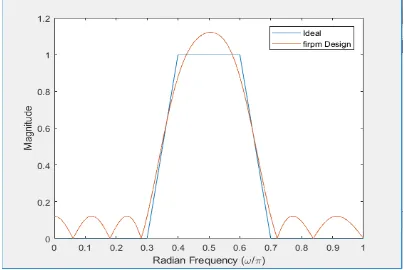
Figure 1.8 Design of equiripple FIR filters using FIRPM

As shown in the above figure, 0.4 is the cut off frequency for the design of the equiripple

bandpass filter. The filter has been designed using Parks Mc Clellan Algorithm which is very

efficient. This reduces the maximum error in each iteration as it is an iterative algorithm. The

MATLAB function firpm is based on Parks McClellan method and is used to design linear

phase FIR filters with a given length and specified passbands and stopbands. The syntax of the

function is shown below:

b=firpm(n,f,a,w)

where n is the filter order, which is one less than the filter length. f and a define the passbands

and stopbands whereas w is the weight vector of length equal to the number of bands.

1.3.4 Difference between equiripple design and least squared FIR filter design

There are two methods available broadly for the design of an efficient and optimal filter design,

(22)

10

equal ripples in the passband and stopband, so the signal distortion which happens at the edge

of the passband is avoided in case of Equiripple Filter Design but it has a large transition width.

On the other hand, the Least Squares Filter design has a smaller bandwidth as compared to

Equiripple filter design, hence the passband width is larger. The passband ripple exhibits a spike

at the passband edge due to Gibb’s phenomenon which causes signal distortion at the edge.

1.3.5 Why are FIR filters preferred over IIR filters?

Table 1.2 Comparison between FIR and IIR filters

1.3.6 General phase FIR filters

GFIR filters also known as General Finite Impulse response filters requires constant group

delay in the system. These filters are asymmetric filters as they do not have same coefficients

on the left and right-hand side, therefore each coefficient is different from the other. The

complexity of the design makes it difficult to optimize and get a good result, so because of this

only the passband delay is taken into account.

A 𝑁𝑡ℎ order general FIR filter [25] consists of (𝑁 + 1) asymmetric impulse responses and can

be represented by a distinct coefficient vector 𝑐 as

𝑐 = [𝑐0, 𝑐1, 𝑐2, 𝑐3, … … . 𝑐𝑁]𝑇 (1.16)

The frequency response of the general FIR filter can be expressed as:

𝐻(𝑤) = ∑ 𝑐𝑛𝑧−𝑛|𝑧 = 𝑒𝑗𝑤𝑇 = |𝐻(𝑤)| 𝑁

𝑛=0 𝑒

𝑗𝜃(𝑤)_(1.17)

The group delay 𝜏(𝑤) of a digital filter can be computed from the derivative of phase 𝜃(𝑤)

with respect to frequency 𝑤 as:

Property FIR filters IIR filters

Phase or group delay Linear phase is always possible

It is hard to design

Stability They are always stable They can exhibit unstable

behavior and limit cycles

Order required Large Small

Implementation Can have multirate or

polyphase implementations

(23)

11

𝜏(𝑤) = −𝜕𝜃(𝑤)

𝜕𝑤 (1.18)

The objective function of the weighted least-squares magnitude response error in a passband

is defined by:

𝑒𝑚𝑝(𝑐) = ∑ 𝑊𝑚𝑝(𝑤𝑖) 𝐼_𝑚𝑝 𝑖 ||𝐻(𝑐, 𝑤𝑖)| − 𝐻𝑑𝑝(𝑤𝑖)| 2 (1.19) 𝑓𝑜𝑟 ∀𝑤𝑖 ∈ 𝜎𝑚𝑝

where 𝐻_𝑑𝑝(𝑤_𝑖) = 1 in the passband, 𝐼_𝑚𝑝 denotes the corresponding number of discrete

frequency points; 𝑊𝑚𝑝(𝑤𝑖) denotes the corresponding frequency error weights, and 𝜎𝑚𝑝

denotes the corresponding union of frequency points of interest.

𝑒𝑚𝑠(𝑐) = ∑ 𝑊𝑚𝑠(𝑤𝑖) 𝐼_𝑚𝑠 𝑖 ||𝐻(𝑐, 𝑤𝑖 )| − 𝐻𝑑𝑠(𝑤𝑖)| 2 (1.20) 𝑓𝑜𝑟 ∀𝑤_𝑖 ∈ 𝜎_𝑚𝑠

where 𝐻_𝑑𝑠(𝑤𝑖) = 0 in the stopband, 𝐼𝑚𝑠 denotes the corresponding number of discrete

frequency points; 𝑊_𝑚𝑠(𝑤_𝑖) denotes the corresponding frequency error weights, and 𝜎_𝑚𝑠

denotes the corresponding union of frequency points of interest.

Similarly, the objective function of the weighted least square errors group delay response error

in the passband is defined by:

𝑒𝑔(𝑐) = ∑ 𝑊𝑔(𝑊𝑖)|𝜏(𝑐, 𝑤𝑖) − 𝜏𝑑(𝑤𝑖)|2 𝐼𝑔

𝑖=0 (1.21)

𝑓𝑜𝑟 ∀𝑤_𝑖 ∈ 𝜎_𝑔

where 𝜏𝑑(𝑤) denotes the desired group delay in the passband; 𝐼𝑔 denotes the number of discrete

frequency points, 𝑊𝑔(𝑤𝑖) denotes the corresponding frequency error weights and 𝜎𝑔 denotes

the corresponding union of frequency points of interest.

The design optimization problem for a general FIR digital filter is to search for an optimal

coefficient vector 𝑐 that simultaneously minimizes its magnitude and group delay errors. For

the case of a lowpass digital filter consisting of a passband and a stopband, a joint objective

(24)

12

𝑒(𝑐) = [𝑚𝑎𝑥 (𝑒𝑚𝑝(𝒄), 𝑒𝑚𝑠(𝒄)) + 𝛼 𝑒𝑔𝑝(𝒄)] 1 2

(1.22)

The parameter 𝛼 denotes a group delay error weighting factor. In this paper, the filter design

problem is formulated as a joint objective function with constraints such that

min

𝑐 𝑒(𝑐)

𝑒𝑚𝑝𝑝(𝑐) ≤ 𝛿𝑚𝑝 𝑓𝑜𝑟 ∀𝑤𝑖 ∈ 𝜎𝑚𝑝

𝑒𝑚𝑠𝑝(𝑐) ≤ 𝛿𝑚𝑠 𝑓𝑜𝑟 ∀𝑤𝑖 ∈ 𝜎𝑚𝑠 (1.23)

𝑒𝑔𝑝(𝑗) ≤ 𝛿𝑔 𝑓𝑜𝑟 ∀𝑤𝑖 ∈ 𝜎𝑔

The parameters 𝑒_𝑚𝑝𝑝(𝑐), 𝑒_𝑚𝑠𝑝(𝑐) 𝑎𝑛𝑑 𝑒_𝑔𝑝 denote respectively passband peak magnitude

error, stopband peak magnitude error, and passband peak group delay error; and the parameters

𝛿_𝑚𝑝, 𝛿_𝑚𝑠 𝑎𝑛𝑑 𝛿_𝑔denote respectively small positive passband magnitude, stopband magnitude,

and group delay tolerance limits. The design problem formulation in (1.19)-(1.22) can be

generalized to the case of a highpass filter or a bandpass filter or a bandstop filter or a

multi-band filter.

1.4 Quantization of coefficients

During the approximation step, the coefficients of the digital filter are calculated with the high

accuracy inherent to the computer employed in the design. When these coefficients are

quantized for practical implementations then the time and frequency responses of the realized

digital filter deviate from the ideal response. In some cases, the quantized filter may even fail

to meet the prescribed specifications. The sensitivity of the filter response to errors in the

coefficients is highly dependant on the type of the structure.

The finite numerical resolution of digital filter representations has an impact on the properties

of filters. The quantization of coefficients, state variables, algebraic operations and signals plays

an important role in the design of recursive filters. Compared to non-recursive filters, the impact

of quantization is often more significant due to feedback process. Several degradations from

the desired characteristics are the potential consequences of a finite word length in practical

implementations.

A recursive filter of the order 𝑁 ≥ 2 can be decomposed into the second-order-sections(SOS).

Due to the grouping of poles/zeros to the filter coefficients with the limited amplitude range, a

(25)

13

𝐻(𝑧) =𝑏0+ 𝑏1𝑧

−1_{+ 𝑏} 2𝑧−2

1 + 𝑎1𝑧−1+ 𝑎2𝑧−2

(1.24)

This can, however, be split into the recursive and non-recursive part. The transfer function of the recursive part of the filter is given below:

𝐻(𝑧) = 1

1 + 𝑎1𝑧−1+ 𝑎2𝑧−2

(1.25)

1.4.1 Initial Coefficient Values for Populations

Let 𝑐_𝑘[𝑢] and 𝑐_𝑘[𝑙] be the upper and the lower bounds for the 𝑘𝑡ℎ coefficient 𝑐_𝑘 of a LP or HP

or BP or BS prototype filter such that:

𝑐_𝑘[𝑙]≤ 𝑐𝑘 ≤ 𝑐𝑘

[𝑢]_{𝑓𝑜𝑟 1 ≤ 𝑘 ≤}𝑁

2 + 1 (1.26)

The initial coefficient 𝑐_𝑝𝑘 for the population member p is computed by:

𝑐𝑝𝑘= 𝑐𝑘 [𝑙]

+ 𝑟𝑎𝑛𝑑 ∗ (𝑐_𝑘[𝑢]− 𝑐_𝑘[𝑙]) 𝑓𝑜𝑟 𝑝 = 1: 𝑃, 𝑘 = 1: 𝐾 (1.27)

Where 𝑟𝑎𝑛𝑑 is the uniformly distributed value between 0 and 1.

1.5 Filter Design Problems

There are basically two classes of digital filters, namely Finite Impulse response (FIR) and

Infinite Impulse response(IIR). Due to the absence of a denominator we find that the FIR filters

are more stable. FIR Filters are guaranteed to be of linear phase with the use of symmetric or

asymmetric coefficients. FIR filters include general phase FIR Filters and Linear Phase FIR

filters in which each of their transfer functions, frequency responses and group delay have been

described earlier in this chapter.

For symmetric filters, there are four types of (𝑀 − 1)𝑡ℎ order linear phase FIR digital Filter of

length M depending on the number of points M of the impulse response and the type of

symmetry.

Impulse response ℎ, distinct coefficient vector 𝑐, the frequency responses 𝐻(𝑐, 𝑤) of Type I

(26)

14

Type I M odd and even symmetry

𝒉 𝒉 = [ℎ(0), ℎ(1), ℎ(2), … . . ℎ(𝑛), ℎ(𝑀 − 2), ℎ(𝑀 − 1)]𝑇

ℎ(𝑛) = ℎ(𝑀 − 1 − 𝑛) 𝑓𝑜𝑟 𝑛 = 0,1,2,3 … . . , (𝑀−3 2 )

𝒄

𝒄 = [𝑐₀, 𝑐₁, 𝑐₂… … 𝑐₍𝑀−1 2 )

] 𝑇

=[ℎ (𝑀−1

2 ) , 2ℎ ( 𝑀−1

2 − 1) , … … . . ,2ℎ(2), 2ℎ(1), 2ℎ(0)] 𝑇

𝐻(𝒄, 𝑤)

𝑒−𝑗(

𝑀−1

2 )𝑤𝑇{ℎ (𝑀−1

2 ) + ∑ 2ℎ(𝑛)𝑐𝑜𝑠 [( 𝑀−1

2 − 𝑛) 𝑤𝑇]

𝑀−3 2

𝑛=0 }

= 𝑒−𝑗(

𝑀−1

2 )𝑤𝑇𝐴(𝑐, 𝑤)

𝐴(𝒄, 𝑤) 𝐴(𝒄, 𝑤) = 𝑐𝑇_{cos 𝑤}

[1 𝑐𝑜𝑠(𝑤𝑇) 𝑐𝑜𝑠(2𝑤𝑇) … … . 𝑐𝑜𝑠 (𝑀−1 2 𝑤𝑇)]

𝑇

The number of impulse responses 𝑀 is related to the filter order 𝑁 by 𝑀 = 𝑁 + 1.

Problem formulation

An 𝑁𝑡ℎ order non-recursive digital filter can be represented by the transfer function

𝐻(𝑧) = ∑ ℎ𝑛𝑧−𝑛 = 𝒄𝑻𝒛(𝑧) (1.28) 𝑁

𝑛=0

Where 𝒄𝑻is the real coefficients vector. N is the total number of filter coefficients.𝑁 − 1 is the

order. For optimization problem, the coefficient vector is:

𝑐𝑇 = [𝑐₁, 𝑐₂… … . 𝑐_𝑛] (1.29)

The frequency response can be gained by substituting 𝑧 = 𝑒𝑗𝑇𝑤 where 𝑇 is the sampling period

in seconds and 𝑤 is the frequency.

For the design of the linear phase FIR digital filter, we assume 𝜎 = 𝑤_𝑖,1 ≤ 𝑖 ≤ 𝑀, be the

group of frequencies to evaluate the frequency response. Therefore the error at each sample

point in 𝑤_𝑖 is given as:

(27)

15

For the symmetric digital filter the group delay is constant which is mentioned as:

𝜏 = 𝑁

2 (1.31)

The main aim of the Filter design problem is to find the optimal coefficient vector c that

minimizes the magnitude and group delay errors. For linear phase, the group delay error is

constant; so it minimizes only the passband and stopband magnitude errors whereas for the

general phase FIR filter the coefficient vector c simultaneously minimizes the magnitude and

group delay errors.

𝑐 = min

𝑐 𝑒(𝑐) (1.32)

For linear phase FIR filter, the minimax objective function 𝑒(𝑐) can be decomposed into

passband magnitude error function 𝑒_𝑝(𝑐) and stopband magnitude error function 𝑒_𝑠(𝑐) as

𝑒(𝑐) = [𝑒_𝑝(𝑐) + 𝑒𝑠(𝑐)] 1_⁄_𝑝

(1.33)

For the general phase FIR filter the joint objective function can be decomposed into passband

magnitude error function 𝑒_𝑚𝑝(𝑐) , stopband magnitude error function 𝑒_𝑚𝑠(𝑐) and group delay

error 𝑒_𝑔𝑝(𝑐) defined by [24] as:

𝑒(𝑐) = [𝑚𝑎𝑥 (𝑒𝑚𝑝(𝑐), 𝑒𝑚𝑠(𝑐)) + 𝛼𝑒𝑔𝑝(𝑐)] 1 2

(1.34)

In this study I have designed four types of linear phase FIR filters of orders 24 and 48. For order

48, the coefficient vector 𝒄will have25 coefficient values whereas for order 24, the coefficient

vector will have 13 values i.e. one more than the order of the filter. This is due to the symmetric

nature of the filter. I have also designed two types of general phase FIR filter of order 24 where

the coefficient vector will have 25 values due to its antisymmetric nature. All the coefficient

values are in the range of -1 to 1.

In the section below, some important deterministic algorithms, heuristic, metaheuristic and

evolutionary algorithms generally used for designing such FIR filter problems have been

described. The objective of each of the algorithms is to minimize the objective error function

(28)

16 1.5.1 Deterministic algorithms

Deterministic digital signal processing is procedure used to display the information in a

measured data. The procedure utilizes different mathematical formulas and implements them

with the help of digital techniques to get appropriate deterministic statistics. Finite impulse

response filter is used in deterministic digital signal processing as a filter with impulse response

to all finite length inputs. It is computed to settle at zero at its finite time.

These algorithms used specific rules for moving from one solution to another. These algorithms

have been successfully applied to many engineering design problems. They always give the

same output, with the underlying machine passing through the same sequence of states.

1.5.2 Heuristic algorithms

The Heuristic search method enhances the capability to explore and exploit locally as well as

globally to obtain optimal design FIR Filter parameters. Heuristic algorithms are superior or

atleast comparable to other algorithms and can be efficiently used for higher order filter designs.

Heuristic algorithms are the algorithms which are designed to solve the problems faster and in

an efficient manner than traditional methods by sacrificing optimality, accuracy, precision or

the completeness for speed. Heuristic algorithms are often employed with the approximate

solutions that are sufficient and the exact solutions that are computationally expensive. The

heuristic algorithms find solutions among all possible ones but they do not guarantee that the

best solution will be found, and therefore they are considered as not-accurate algorithms.

Approximate algorithms entail the interesting issue of quality estimations of the solution they

find. These problems can be a real challenge in solving strong mathematical problems. The

main goal of the heuristic algorithms is to find as good solution as possible to all instances of

the problem.

Usually, heuristic algorithms are used for problems that cannot be solved [1]. Classes of time

complexity are defined to distinguish the problems according to their hardness. Turing

machines are an abstraction that is used to formulate the notion of the algorithm and also its

computational complexity. Class P consists of those problems that are solved on a deterministic

turing machine in polynomial time. Class NP consist of all those problems whose solution can

be found in polynomial time on a non-deterministic Turing machine. A subclass of NP, Class

NP-complete includes problems such as a polynomial algorithm for solving one of them can be

(29)

17

can be understood as the class of problems that are NP-complete or harder. Some of the heuristic

algorithms are:

Swarm intelligence which employs a large number of agents interacting locally with one

another and the environment.

Tabu Search which uses dynamically generated tabus to guide the solution search to optimum

solutions. It examines the potential solution to the problem and checks the local intermediate

neighbours to find the improved solution.

Simulated Annealing is used in global optimization to give a reasonable approximation of a

global optimum in a function for the search space.

1.5.3 Metaheuristic algorithms

Metaheuristic algorithms are basically higher level heuristic algorithms which are used for IIR

filter designs. The term ‘meta’ means higher-level or beyond , so metaheuristic means literally

to find the solution using higher-level techniques. They are considered as higher-level

techniques or strategies which intend to combine with lower level techniques for exploration

and exploitation of the huge space for parameter search when used in filter design problems.

Metaheuristic algorithms are a combination of heuristic and randomization. It is formally

defined as an iterative generation process which guides a subordinate heuristic by combining

the different concepts intelligently for exploring and exploiting the search space. The main goal

of metaheuristics is to efficiently explore the search space in order to find the optimal solutions.

The techniques which constitute the metaheuristic algorithms range from the simple local

search procedures to complex learning processes. Metaheuristic algorithms are

non-deterministic algorithms. They incorporate mechanisms to avoid getting trapped in the confined

areas of the search space.

Metaheuristics are not problem specific. They usually make use of the domain-specific

knowledge in the form of heuristics that are controlled by the upper level-strategy. Today’s

more advanced metaheuristics make use of the search experience to guide the search. The

metaheuristic is a general algorithm framework for addressing the interactable problems.

Metaheuristics are approximation algorithms that cannot always produce provably optimal

solutions but they do have the potential to produce good solutions in a reasonable amount of

(30)

18 1.5.4 Evolutionary algorithms

Evolutionary Algorithms are used in finding the solution for problems where there is no explicit

solution and that is what is exactly required for digital filter design problem. Their particular

strength is that they can efficiently search for a solution in a very large space.

Evolutionary Algorithms(EA) consist of several heuristics, which are able to solve optimization

tasks by initiating some aspects of natural evolution. They may use different levels of

abstraction, but they are always working on the populations of possible solutions for a given

task. Evolutionary methods are used in hard optimization problems rather than pattern

recognition.

1.5.4.1Genetic algorithms

In nature, every living organism has a set of rules, a blueprint so to speak and describing how

the organism is created. The genes of an organism represent these rules and are connected

together into long strings called chromosomes. Each gene represents the specific property of an

organism and the collective set of gene settings are referred to as organism’s genotype. The

physical expression of the genotype is called the phenotype. Yet in rare cases, it will be

expressed in the organism as a completely new trait. It is a local search technique used to find

approximate solutions to optimization and search problems. Genetic algorithms are a particular

class of Evolutionary algorithms that use techniques inspired by evolutionary biologies such as

inheritance, mutation, selection, and crossover. They are typically implemented as a computer

solution in which a population of abstract representations of candidate solutions to an

optimization problem evolves towards better solutions. The evolution normally starts from a

population of completely random individuals and occur in generations. In each generation the

fitness of the whole population is evaluated, multiple individuals are stochastically selected

from the current population and modified to form a new population. The new population is then

used in the next iteration of the algorithm. Genetic Algorithms uses crossover and mutation as

a search mechanism. Some applications of genetic algorithms are as follows:

1) Automotive design

2) Engineering design

3) Robotics

4) Evolvable hardware

(31)

19

1.5.4.1Differential evolution

In evolutionary computation, differential evolution is a method that optimizes a problem by

iteratively trying to improve a candidate solution with regard to a given measure of quality.

Here each variable’s value is represented by a real number. Differential Evolution is a design

tool of great utility that is accessible for practical applications. DE has been used in several

scientific and engineering applications to discover effective solutions to nearly intractable

problems without appealing to expert knowledge or complex design problems. If a system is

amenable to be rationally evaluated, DE can provide the means for extracting the best possible

performance from it. The Differential Evolution uses mutation as a search mechanism and

selection to direct the search towards the prospective regions in the feasible region. DE is a

population based search technique which utilizes NP variables as a population of D dimension

parameter vectors for each generation. The initial population is chosen randomly. In the case of

the available preliminary solution, the initial population is generated by adding normally

distributed random deviations to the preliminary solutions. The basic idea behind DE is a new

scheme for generating trial parameter vectors. If the resulting vector yields a lower objective

function value than the predetermined population member, the newly generated vector replaces

the vector with which it was compared. The best parameter vector is evaluated for every

generation in order to keep track of the progress that is made during the optimization process.

DE maintains two arrays each of which holds a population size NP and D dimensional

real-valued vectors. The primary array holds the current vector population, while the secondary

array accumulates vectors that are selected for the next generation.

(32)

20

The above table shows that for the Multimodal Separable functions, the Differential Evolution

(DE) and Harmony Search (HS) algorithms are a very efficient method for finding the optimal

solution and its convergence speed is much faster than the Particle Swarm optimization.

1.6 Neural Networks

A neural network is a massively parallel structure which is composed of many nonlinear

processing elements connected to each other through weights. It is a trainable nonlinear

dynamic system which stores various patterns with distributed coding. When compared with

sequential digital computers, we find that neural networks have a faster response due to parallel

processing and a higher performance due to nonlinear processing.

Neural networks basically have a multilayer structure consisting of a sigmoidal type of

nonlinear operation at the output of each hidden neuron and the output of each output neuron.

Neural network classifiers are free model estimators. They usually do not provide assumptions

on how the outputs depend on the inputs. Instead, they decide the boundaries of the classes and

adjust themselves to the training set by the learning algorithm.

1.7 Contributions

The main contribution of the work done here is the implementation of HS Algorithm and

adapting the algorithm to utilise it in designing FIR filters and neural networks. The algorithm

has been initially used for several other applications mentioned in Chapter 2. The disadvantage

of the other algorithms like GA and PSO is that they require fine tuning of parameters in order

to obtain a feasible solution. Also, diversification and intensification are the two major

components whose balanced combination is very important for the success of any metaheuristic

algorithm. Harmony search successfully balances these two major components by pitch

adjustment and harmony considering rate and therefore it ensures a certain level of efficiency

and that the evolving system will not get trapped in the local minima.

1.8 Motivation and Outline of Thesis

The main objective of this project is the requirement of an efficient optimization algorithm that

will be able to optimize complex designs problems such as for the advanced digital filters and

neural networks making the filter processes much more efficient and noise free. Since the

algorithm produced some effective results in the initial runs, hence it motivated me to explore

(33)

21

with those already present algorithms. The coefficient values have to be optimized using an

optimization algorithm for reducing the noise to the minimum and designing a good filter for

real time applications. Likewise, for designing complex neural networks optimization algorithm

plays a vital role in determining the weights and bias of the network. The weights and bias are

the important optimization aspects which helps to reduce the error between the actual output

and the desired output in such a way that the neural network will give the same output even by

introducing some amount of noise at the input. There are some algorithms based on

evolutionary methods which can design digital filters with comparatively less time. Various

types of complex neural network designs have been adopted from [18] in my thesis which

includes two layers neural network using XOR, Advanced feedforward neural networks (0-9)

digit and also the two layer neural network design results for fuzzy inference networks.

The thesis clearly presents Harmony Search algorithm and its applications in designing the

advanced digital filter designs and neural network problems.

The first chapter illustrates the theory about the digital filters, the various types of digital filters,

the comparison between the two types and details about the types of filters have also been

described. The conventional methods used for designing filters and common strategies used for

the same have also been highlighted in Chapter 1. It basically contains the main goals of the

thesis.

In the second chapter, some of the state of art of methods for designing the FIR digital filter

designs are discussed and the literature has been reviewed. The Harmony Search Algorithm, its

pros and cons, strengths and weakness along with the improvements and the basic introduction

to neural networks have been discussed in Chapter 2.

The third Chapter describes the methodology or the creation of work required to obtain each of

the Neural Networks and filter design results mentioned in the Chapter 4.

Chapter 4 shows the evidences that the harmony search Algorithm can be used as a good

alternative to the Parks McClellan algorithm through the results which have been shown.

(34)

22

Review of Literature

Digital filtering is a ubiquitous operation in digital signal processing applications and is realized

using infinite impulse response(IIR) or Finite impulse response(FIR) filters. Although FIR

Filter requires a large number of coefficients when compared to the IIR Filters, it is compared

to IIR Filters due to stability and phase linearity properties.

An optimization algorithm is a procedure which is executed iteratively by comparing various

solutions to an optimum solution is found. The main objective of an optimization algorithm

could be simply to minimize the cost of production and to maximize the efficiency of the of the

production. In an optimal problem formulation, the optimal design is achieved by comparing

few alternative solutions. In this particular method, the feasibility of each design solution is first

investigated. Therefore, an estimate of underlying objective of each solution is compared with

the others and the best solution is recorded. The design parameters, however, can vary from

product to product. The purpose of the formulation is to create the mathematical model of the

optimal design problem, which can be solved using optimization algorithm.

The formulation of optimization algorithm begins with identifying the design variables which

are primarily varied during the optimization process. The design problem involves many design

parameters, of which some are highly sensitive to the proper working of the design. These

parameters are known as the design variables. The constraints represent some functional

relationships among the design variables and parameters satisfying certain physical

phenomenon and certain resource limitations. There are mainly two types of constraints:

Inequality constraints and Equality constraints.

The learning problem in neural networks is formulated in terms of minimization of a loss

function. The function is composed of error and regularization terms. The error term mainly

evaluates how the neural network problem fits the data set. The regularization is used to prevent

overfitting, by controlling the effective complexity of the neural network design. The loss

function depends on adaptive parameters (bias and synaptic weights) of the neural network. We

can group them conveniently into a single n-dimensional weight vector w. There are many

training algorithms that can be used in the training process of the neural network.

In this thesis study, I have made use of the Harmony Search Algorithm to solve the complex

(35)

23

digital filter designs which can be used for many real-time applications. Digital filters are an

essential part and one of the most important features of modern day circuit designs and plays a

vital role in the improvement of the overall system by producing better results. Harmony Search

Algorithm is just a successful example which transforms the qualitative improvisation process

into some quantitative rules by idealization, thus turning the beauty and harmony of music into

an optimization procedure through a search for a perfect harmony.

2.1 Survey of Harmony Search Applications

In the real world, modern science and industry are rich in the problems of optimization. HS was

originally proposed by Geem [2] and applied to solve the optimization problem of water

distribution networks in 2000, the applications of the HS have covered many areas including

industry, optimization benchmarks, power systems, medical science, control systems,

construction design, and information technology [3].

The Industry is a prominent area full of various practical optimization issues subject to

multi-modal, constrained, nonlinear, and dynamical. The HS algorithm proposed by Saka [4]

determines the optimal steel section designations from the available British steel section table

and implements the design constraints from BS5950. Recently, an enhanced harmony search

(EHS) in [5] is developed enabling the HS algorithm to quickly escape from local optima. The

proposed EHS algorithm is utilized to solve four classical weight minimization problems of

steel frames including two-bay, three-storey planar frame subject to a single-load case, onebay,

ten-storey planar frame consisting of 30 members, three-bay, twenty-four storey planar frames,

and Spatial 744 member steel frame. In [6], the HS is used to select the optimal parameters in

the tuned mass dampers [6]. Fesanghary et al. [7] propose a hybrid optimization method based

on the global sensitivity analysis and HS for the optimal design of shell and tube heat

exchangers. There is a lot of work focused on the optimization issues concerning power

systems, such as cost minimization. A modiﬁed HS algorithm is proposed to handle non-convex

economic load dispatch of real-world power systems. The economic load dispatch and

combined economic and emission load dispatch problems can be converted into the

minimization of the cost function [8]. Sinsuphan et al. [9] combine the HS with sequential

quadratic programming and GA to solve the optimal power ﬂow problems. The objective

function to be optimized is the total generator fuel costs in the entire system. The chaotic

self-adaptive differential HS algorithm, proposed by Arul et al. [10], is employed to deal with the

(36)

24

factor to adjust the bandwidth (bw). With this modiﬁed HS, they develop a pre-training process

to select the weights used in the combining of feature maps to make the target more conspicuity

in the saliency map. In their method based on the HS, Fourie et al. [12] design a harmony ﬁlter

using the improved HS algorithm for a robust visual tracking system.

2.2 What is Harmony Search Algorithm?

Harmony Search Algorithm is an emerging metaheuristic algorithm that was inspired by the

observation that the aim of music is to search for a perfect state of harmony. There is a parallel

idea between HS and how the Jazz musicians create harmony when they play music.

HS algorithm is based on a few parameters: hmcr, par, and bw. The parameter hmcr is called

the Harmony memory considering rate and it denotes the rate of choosing candidates from the

Harmony Memory(HM) and generally ranges from 0.7 to 1. The parameter par is called the

pitch adjusting rate and indicates the rate of choosing the neighboring value and can be selected

from 0 to 1. The parameter bw is called the bandwidth denotes the amount of maximum rate of

change of change in the pitch adjustment.

2.3 Design of Harmony Search Algorithm

This section discusses the projected effective harmony Search. Initially a brief outline about HS

is given and lastly, the alteration procedures of the proposed effective Harmony Search are

discussed.

Harmony Search Algorithm is one of the efficient optimization algorithm developed by Geem

et al. [13]. It is inspired by the music improvisation process. The analogy between music

improvisation and optimization can be established by creating a correspondence between music

player to the decision variable. In order to execute the technique in real time optimization each

decision variable chooses and possible range together to make a solution. This solution is then

improved by creating harmony memory, and pitch adjusting. Over the year various optimization

algorithms [14-16] are proposed but HSA remains one of the best choices for function

optimization. In order to introduce the HS algorithm for engineering optimization. [17].

The various involved in Harmony Search algorithm are discussed as follows [13]:

Step 1 Initialize harmony memory.

(37)

25

Step 3 Update Harmony Memory.

Step 4 Check Stopping criterion.

During optimization, harmony search algorithm attempts to find the harmony vector x which

minimizes (or maximizes) a specified objective function 𝑓(𝑥). The algorithm consists of four

steps which are described below:

The above four steps are discussed in the following subsections [1]-[4] [18]:

1. Initialize the harmony memory: In this step, each parameter 𝑚 for 𝑚 = 1 𝑡𝑜 𝑀 of

each of the 𝑃 initial harmony vectors 𝑥_𝑝 = [𝑐_𝑝1, 𝑐_𝑝2, 𝑐_𝑝3, … . , 𝑐_𝑝𝑚] for 𝑝 = 1 𝑡𝑜 𝑃 is

generated randomly within the upper limit 𝑢 and the lower limit 𝑣 of the 𝑚𝑡ℎ parameter

as:

𝑐_𝑝𝑚 = 𝑣 + 𝑟𝑎𝑛𝑑 ∗ (𝑢 − 𝑣) 𝑓𝑜𝑟 𝑝 = 1 𝑡𝑜 𝑃 𝑎𝑛𝑑 𝑚 = 1 𝑡𝑜 𝑀 (2.1)

The harmony memory consisting of 𝑥𝑝 for 𝑝 = 1 𝑡𝑜 𝑃 are arranged in the ascending

order of increasing objective function 𝑓(𝑥_𝑝) for 𝑝 = 1 𝑡𝑜 𝑃 such that 𝑓(𝑥₁) ≤ 𝑓(𝑥₂) ≤

𝑓(𝑥₃) … . ≤ 𝑓(𝑥𝑝) as:

[

𝑐₁₁ ⋯ 𝑐_1𝑝

⋮ ⋱ ⋮

𝑐𝑝1 ⋯ 𝑐𝑝𝑚

] (2.2)

2. Improvising a new solution- In this step, HS improvises 𝑄 harmony vectors 𝑥𝑚′ =

[𝑐_𝑞1′ , 𝑐_𝑞2′ , 𝑐_𝑞3′ , … . . , 𝑐_𝑞𝑚′ _{] 𝑓𝑜𝑟 𝑞 = 1 𝑡𝑜 𝑄}_{based on two considerations, namely memory}

considerations and pitch adjustment.

For the memory consideration, each parameter value 𝑐_𝑞𝑚′ _for_{𝑚 = 1 𝑡𝑜 𝑀}_{of the new}

harmony vector is randomly selected among the corresponding 𝑃 parameter values

{𝑐_1𝑚, 𝑐_2𝑚, 𝑐_{3𝑚,……..,}𝑐_𝑝𝑚} with a probability 𝐶 ∈ [0,1].

𝑐_𝑞𝑚′ = {𝑐𝑞𝑚 ′ _{∈ {𝑐}

1𝑚, 𝑐2𝑚, 𝑐3𝑚, … , 𝑐𝑝𝑚} 𝐶 ∈ [0,1] (2.3𝑎) 𝑐_𝑞𝑚′ _{= 𝑐}

𝑞𝑚′ (𝑜𝑙𝑑) (2.3𝑏)

For the pitch consideration, an additional search for good harmony in the search space

is achieved by adjusting each continuous parameter 𝑐_𝑞𝑚, in a new solution vector at a pitch

adjusting rate (𝐴) for 𝐴 ∈ [0,1] as

𝑐_𝑞𝑚′ = {𝑐𝑞𝑚

′ _{+ 𝑟𝑎𝑛𝑑𝑛 ∗ 𝑏𝑤 (2.4𝑎)}

(38)

26

where 𝑟𝑎𝑛𝑑𝑛 is the normally distributed pseudorandom numbers and 𝑏𝑤 is an arbitrary

distance bandwidth which determines the maximum change to each parameter of the new

harmony vector.

The upper and lower bound are applied to each parameter of each of the 𝑄 new harmony vectors

such that:

Replace any new parameter 𝑐_𝑞𝑚′ < 𝑣 (2.5𝑎)

Replace any new parameter 𝑐_𝑞𝑚′ _{> 𝑢 (2.5𝑏)}

3. Harmony Memory Update: In order to update the population with 𝑄 new harmony vectors

𝑥_𝑞′ = [𝑐_𝑞1, , 𝑐_𝑞2′ , 𝑐_𝑞3′ , … , 𝑐_𝑞𝑀′ ] for 𝑞 = 1 𝑡𝑜 𝑄, the objective function 𝑓(𝑥_𝑞′) of each of the

harmony vectors is calculated. Among the 𝑃 existing harmony vectors and 𝑄 new harmony

vectors, the top 𝑃 harmony vectors based on the ranking of their objective functions are

selected for next improvisation.

4. Stopping criterion: The improvisation process in steps 3 and 4 is terminated when the

maximum number of improvisations is reached. Finally, the best harmony memory vector

𝑥𝑏𝑒𝑠𝑡 is selected among all the harmony vectors to be the solution for the optimization

problem.

𝒙𝒃𝒆𝒔𝒕 _{∈ (𝒙}

𝟏, 𝒙𝟐, 𝒙𝟑… … 𝒙𝒑) (2.6)

2.4 Improvements in Harmony Search Algorithm

Because the effects of optimization are mostly depended on the initialization of HM, the

selection of parameters such as HMCR and the new ways of solution. So, if the harmony search

algorithm faces with bad optimization or unsuitable parameters selection or complex

optimization objective, some shortage such as weak local searching ability and convergence

precision will appear. Since the harmony search algorithm was invited, some experts put

forward many effective suggestions to improve the algorithm, which include two aspects, one

is improving algorithm itself (including HM parameters optimization) and other is combining

with other algorithms.

Basic Harmony Search Algorithm uses fix value for PAR and BW and initializes these

parameters in step 1, and these parameters cannot be updated in the iterative process. Because

the small PAR and big BW results in bad algorithm effect, so it needs to add definite iterative

(39)

27

In 2007, Mahdevi put forward the Improved Harmony Search Algorithm(IHS), it brought

forward the dynamic adaptive PAR and BW strategy, and the two parameters can vary

dynamically between maximum and minimum, while the PAR was increasing linearly with the

number of iterations and the BW index decreasing with the number of iterations.

𝑃𝐴𝑅(𝑔𝑛) = 𝑃𝐴𝑅𝑚𝑖𝑛+

(𝑃𝐴𝑅𝑚𝑎𝑥 − 𝑃𝐴𝑅𝑚𝑖𝑛)

𝑁𝐼 × 𝑔𝑛 (2.7)

Where,

𝑃𝐴𝑅(𝑔𝑛) = Pitch Adjusting Rate for each generation

𝑃𝐴𝑅_𝑚𝑖𝑛= Minimum Pitch Adjusting Rate

𝑃𝐴𝑅𝑚𝑎𝑥 = Maximum Pitch Adjusting Rate

𝑁𝐼 = Number of Solution vector generation

𝑔𝑛 = Generation Number

𝑏𝑤(𝑔𝑛) = 𝑏𝑤𝑚𝑎𝑥𝑒𝑥𝑝(𝑐. 𝑔𝑛) (2.8)

𝑐 =

𝑙𝑛 (_𝑏𝑤𝑏𝑤𝑚𝑖𝑛 𝑚𝑎𝑥)

𝑁𝐼 (2.9)

2.5 Why is Harmony Search successful?

Presently in the event, when we compare HS with other metaheuristic algorithms, we can

recognize its methods for taking care of intensification and diversification in the HS system,

and presumably, comprehend why it is an exceptionally fruitful metaheuristics calculation. In

the HS calculation, diversification is basically measured by the pitch adjustment and

randomization [19]. In this case, there are two subcomponents for diversification, which may

be an essential component for high proficiency of the HS strategy. The principal subcomponents

of making new music or creating new arrangements by means of randomization would be in

any event at the same level of effectiveness as different calculations by randomization. In any

case, an extra subcomponent for Harmony search diversification is the pitch adjustment. Pitch

adjusting is carried out by adjusting the pitch in the given bandwidth by a small random amount

relative to the existing pitch or solution from the harmony memory. Pitch adjustment is the