University of Windsor University of Windsor
Scholarship at UWindsor
Scholarship at UWindsor
Electronic Theses and Dissertations Theses, Dissertations, and Major Papers
1-12-2016
Improving Spatially Distributed Multiagent Pathfinding Using
Improving Spatially Distributed Multiagent Pathfinding Using
Cooperative JPS
Cooperative JPS
Sanjay Renukamurthy
University of Windsor
Follow this and additional works at: https://scholar.uwindsor.ca/etd
Recommended Citation Recommended Citation
Renukamurthy, Sanjay, "Improving Spatially Distributed Multiagent Pathfinding Using Cooperative JPS" (2016). Electronic Theses and Dissertations. 5663.
https://scholar.uwindsor.ca/etd/5663
This online database contains the full-text of PhD dissertations and Masters’ theses of University of Windsor students from 1954 forward. These documents are made available for personal study and research purposes only, in accordance with the Canadian Copyright Act and the Creative Commons license—CC BY-NC-ND (Attribution, Non-Commercial, No Derivative Works). Under this license, works must always be attributed to the copyright holder (original author), cannot be used for any commercial purposes, and may not be altered. Any other use would require the permission of the copyright holder. Students may inquire about withdrawing their dissertation and/or thesis from this database. For additional inquiries, please contact the repository administrator via email
IMPROVING SPATIALLY DISTRIBUTED
MULTIAGENT PATHFINDING USING
COOPERATIVE JPS
By
SANJAY RENUKAMURTHY
A Thesis
Submitted to the Faculty of Graduate Studies
Through the School of Computer Science
In Partial Fulfillment of the Requirements for
the Degree of Master of Science at the
University of Windsor
Windsor, Ontario, Canada
2016
Improving Spatially Distributed Multiagent Pathfinding using Cooperative JPS
by
Sanjay Renukamurthy
APPROVED BY:
______________________________________________ Dr. Myron Hlynka, External Reader
Department of Mathematics and Statistics
______________________________________________ Dr. Imran Ahmad, Internal Reader
School of Computer Science
______________________________________________ Dr. Scott Goodwin, Advisor
School of Computer Science
iii
DECLARATION OF ORIGINALITY
I hereby certify that I am the sole author of this thesis and that no part of this
thesis has been published or submitted for publication.
I certify that, to the best of my knowledge, my thesis does not infringe upon
anyone’s copyright nor violate any proprietary rights and that any ideas, techniques,
quotations, or any other material from the work of other people included in my thesis,
published or otherwise, are fully acknowledged in accordance with the standard
referencing practices. Furthermore, to the extent that I have included copyrighted
material that surpasses the bounds of fair dealing within the meaning of the Canada
Copyright Act, I certify that I have obtained a written permission from the copyright
owner(s) to include such material(s) in my thesis and have included copies of such
copyright clearances to my appendix.
I declare that this is a true copy of my thesis, including any final revisions, as
approved by my thesis committee and the Graduate Studies office, and that this thesis
iv
ABSTRACT
The Multiagent Pathfinding problem (MAPF) applies in fields such as video
games, robotics, warehouse management, etc. MAPF is mainly concerned with
routing units while avoiding collision. A recent approach by Wilt et al. to MAPF for
maps with narrow corridors spatially partitions maps into High Contention (HCA) and
Low Contention areas (LCA). A modified Cooperative A* is used in LCA.
In our approach we introduce a new algorithm by combining “Cooperative”
and “Jump Point Search” (JPS) to traverse through the LCA. JPS is modified to
handle the multiagent environment by incorporating a new stopping rule to identify
between HCA and LCA called “forced selection”. As JPS jumps from node to node,
we introduce a “backtracking mechanism” to avoid collision. We evaluate our
algorithm against Wilt et al.’s algorithm on real video game maps and demonstrate
v
DEDICATION
To my loving family:
Father: Renuka murthy
Mother: Kavitha
Brother: Ajay
vi
ACKNOWLEDGEMENTS
I would like to thank my supervisor, Dr. Scott Goodwin, for giving me the
opportunity to get an exposure of the research field. It has been a great experience
working under his guidance. His constant motivation, support and faith guided me in
successful completion of my thesis.
I would like to thank my internal reader Dr. Imran Ahmad for his support and
showing interest towards my research. I am also thankful to my external reader Dr.
Myron Hlynka for being flexiable about the schedule time of my defence.
I give my sincere thanks to Mrs. Karen Bourdeau, the graduate secretary, who
always supported and helped me when ever I needed any assistance in various
academic issues and providing a GA position.
Lastly, I would like to thank my family and friends for their utmost faith in me
and for supporting me through the ups and downs of my life.
vii
TABLE OF CONTENTS
DECLARATION OF ORGINALITY………...…………iii
ABSTRACT………...…………..iv
DEDICATION………...………...v
ACKNOWLEDGEMENTS………...……….vi
LIST OF TABLES………..…….x
LIST OF FIGURES………....xi
LIST OF ALGORITHMS………..………….xiv
LIST OF ACRONYMS….………..…………...xv
CHAPTER-1 INTRODUCTION………..…………..1
1.1 Graph Representation of Maps ………...….2
1.1.1 Grids………..…3
1.1.1.1 Regular Grids……..………...3
1.2 Heuristic………... ………...4
1.2.1 Manhattan Distance………..…4
1.2.2 Euclidean Distance………...……….5
1.3 Search Algorithms ………..……….6
viii
1.3.2 Multiagent Pathfinding………...…...………8
1.4 Problem Statement….………..……….…….10
1.5 Motivation ……..………..……….10
1.6 Thesis Claim…..……….11
1.7 Thesis Outline…..………...………11
CHAPTER-2 RELATED WORK………...…..13
2.1 Single Agent Pathfinding Algorithms………..…...…...…13
2.1.1 A*………...……….13
2.1.2 Jump Point Search……….………...…...13
2.2 Multi-Agent Pathfinding Algorithms………...19
2.2.1 Decentralized Approach…………...……….…...…...19
2.2.2 Centralized Apprach……….………...24
2.3 Summary………27
CHAPTER-3 SPATIALLY DISTRIBUTED MULTIAGENT PATH PLANNING……….28
3.1 Spatial Distribution of Map………....…...………...28
3.2 High Contention Area…….………...………..………...30
3.3 Low Contention Area…….………...………..32
3.4 Spatiallly Distributed Algorithm.………...……….………...33
ix
CHAPTER 4 PROPOSED APPROACH……….35
4.1 Cooperative JPS.………..…..………..…...35
4.1.1 Backtracking Mechanism………….……….….…...36
4.1.2 Forced Selection………...……….………..…....38
4.1.3 Collision Avoidance………..……...……….…..…....40
4.1.4 High level Path using JPS……….…..…....43
4.2 Summary………..………...44
CHAPTER-5 EXPERIMENTAL SETUP AND RESULTS.………..45
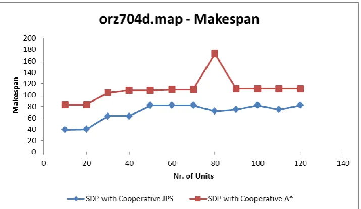
5.1 orz704d.map..…………..…..………...…………...46
5.2 den204d.map..…………..…..………..………...48
5.3 den401d.map..…………..…..……….………...51
5.4 orz704d.map..…………..…..………..………...55
5.5 Summary………..…..………..…………...56
CHAPTER-8: CONCLUSION AND FUTURE WORK………...…...57
REFERENCES……….…..59
APPENDIX 1………..………..…………...………...62
x
LIST OF TABLES
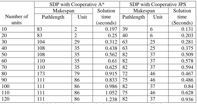
1a Makespan and Solution time on map orz704d.………..….47
1b Number of failed units on map orz704d………. 48
2a Makespan and Solution time on map den204d ………....………...…50
2b Number of failed units on map den204d ………..………..…51
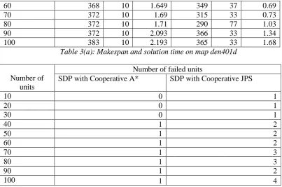
3a Makespan and Solution time on map den401d………...….53
3b Number of failed units on map den401d……….………... 53
4a Makespan and Solution time on map den505d ………....………...55
xi
LIST OF FIGURES
1 Single agent path on a video game [1] ………….……….….………1
2 Two routes for Truck driver from start point ‘Denver’ to destination ‘Ohio’[2]………..………2
3a 4-way movement on square grid………...………4
3b 8-way movement on square grid………...………4
4 Search path calculated using Manhattan distance ………..……..……..5
5 Search path calculated using Euclidean distance ………..…….6
6 Working diagram of A* algorithm ……….……….…..…...16
7a Straight pruning rule………..……….….17
7b Diagonal pruning rule………..…..……….….17
8 Forced neighbor for straight move……….………..….18
9 Forced neighbor for diagonal move……….……….19
10a Cooperative A* without collision……….………...…..21
10b Cooperative A* with collision……….………...21
11 Passage with path ‘A’ and ‘B’ [17].………....24
12 Spatial distribution of map into controllers and transition move between controllers and internal move ……….29
13 High level paths for units U1 and U2………..………29
14a 2 wide central core HCA………...30
14b 3 wide central core HCA………...30
14c 4 wide central core HCA………...30
15 High Contention Area [18]………..………31
16 Backtracking mechanism example……….……….38
xii
18a Diagonal side-way movement……….………..41
18b Straight horizontal side-way movement……….……...41
19 High level path using JPS for two units on SDP framework…..…...44
20a Makespan generated for SDP with Cooperative JPS and
SDP with Cooperative A* on map orz704.map………46
20b Solution time generated for SDP with Cooperative JPS and
SDP with Cooperative A*on orz704d map………...47
20c Number of Failed units for SDP with Cooperative JPS and
SDP with Cooperative A*on map orz704d over each instances………...47
21a Makespan generated for SDP with Cooperative JPS and
SDP with Cooperative A* on map den204d map……….……….49
21b Solution time generated for SDP with Cooperative JPS and
SDP with Cooperative A*on den204d map…….………...49
21c Number of Failed units for SDP with Cooperative JPS and
SDP with Cooperative A*on map den204d over each instances………..49
22a Makespan generated for SDP with Cooperative JPS and
SDP with Cooperative A* on map den401d map……….……….51
22b Solution time generated for SDP with Cooperative JPS and
SDP with Cooperative A*on den401d map….……….……52
22c Number of Failed units for SDP with Cooperative JPS and
SDP with Cooperative A*on map den401d over each instances……….…...…...52
23a Makespan generated for SDP with Cooperative JPS and
SDP with Cooperative A* on map den505d map……….……….54
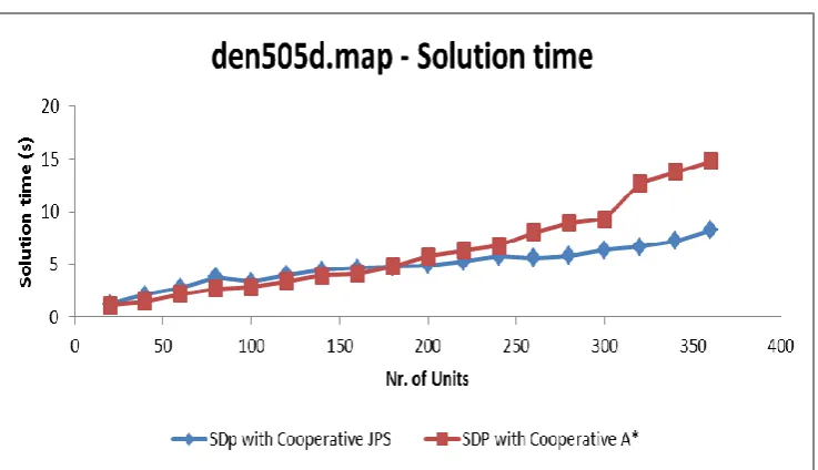
23b Solution time generated for SDP with Cooperative JPS and
xiii
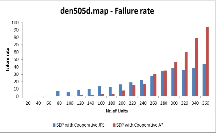
23c Number of Failed units for SDP with Cooperative JPS and
xiv
LIST OF ALGORITHMS
1 Low Contention Area accepting unit [18]……….33
2 High Contention Area accepting unit [18]……….………..………….34
3 Bactracking mechanism in Cooperative JPS………...…………..37
4 Forced Selection in Cooperative JPS………..…………..39
5 Collision Avoidance in Cooperative JPS………..…………42
xv
LIST OF ACRONYMS
JPS – Jump Point Search
RTS – Real Time Strategy
NPC – Non Player Control
GPS – Golbal Positioning System
MAPF – Multiagent Pathfinding
CBS – Conflict Based Search
CT – Conflict Tree
LRA* - Local Repair A*
COWHCA* - Conflict Orientented Windowed Hiearchical Cooperative A*
WHCA* - Windowed Hiearchical Cooperative A*
RWT – Reduced Wait Time
SDP – Spatially Distributed Pathfinding
HCA – High Contention Area
LCA – Low Contention Area
DM – Direction Map
DV – Direction Vector
MV – Movement Vector
OD – Operator Decomposition
ID – Independence Detection
MGS – Maximum Group Size
HCA* - Hierarchical Cooperative A*
ICTS – Increasing Cost Tree Search
SPP – Simple Pairwise Prusing
xvi
REPP – Repeated Enhanced Pairwise Prusing
1
CHAPTER 1: INTRODUCTION
Pathfinding problem can be found in many fields from video game industry to ware
house management. The general problem which is addressed here is to find an optimal
path for a unit from its start node to goal node on a graph representation of map.
Based on application in use, the above problem statement can be used for different
usage such as in field of video game they require the problem to be solved in
minimum time, but in other application such GPS, the problem would be to find a safe
and short to the goal. Consider a scenario in one of the Real Time Strategy (RTS)
games, where the Non Player Control (NPC) has to find a path from its start to goal
position real quickly to give a realistic feel to the gamer while playing. In figure 1, a
NPC unit as to travel from tower to its house, so the start position is tower and goal
position is house. Even though the unit could have travel through the river, but that
would not be a realistic path. So the unit crosses the bridge and reaches its destination.
In here we want an algorithm which could solve the pathfinding problem quickly.
Figure 1: Single agent path on a video game [1]
Similarly we could find the same problem with different objective for solving in
application like GPS. Consider the figure 2, where a vehicle has to travel from Denver
2
route2 is shorter compared to route1 the driver takes a longer route1 because it’s safer
then shorter route2. In this case the main criterion of finding the path from Denver to
Ohio is to find a safest path rather than shortest path.
Figure 2: Two routes for Truck driver from start point ‘Denver’ to destination ‘Ohio’ [2]
The three basic elements used to solve a pathfinding problem in any of the fields
are graph representation of map, heuristic to guide the unit to goal and a search
algorithm to find the route for the unit.
1.1Graph representation of map:
The maps can broadly divided into grids and hierarchical techniques that are
widely used in many real world applications to find path. Map represented as grids
consists of polygons grouped together to form a map. Consider a graph G(V, E) where
V is set of vertices and E is set of edges. The continuous connected graph G, can be
represented by placing a vertex at the centre of polygon or at each of its corners. In a
map where the vertex is at the center of polygon, the edges would be the connection
between polygons and in case where vertex is at the corners, the edges can be sides of
the polygon. The only disadvantage of using a grid over hierarchical techniques is that
3
1.1.1 Grids
Grids are connected graph with vertices and edges to represent a map. Each of
the polygon on the map is called as the tile/node based on the application it is being
used. There are two popular grid representation firstly regular grids where all the
nodes are formed using the same kind of polygons and irregular grids where the map
could be represented with different types of polygons.
1.1.1.1Regular Grids
Regular grids are the ones where the entire maps are represented using
uniformed polygons such as square, hexagon and triangle. The regular grids are one
of the famous map representations which are used in many fields like video games
such as Pac-man, Pokémon games, sim city etc. and robotics where the mars rover
robots used regular grids for their exploration [3]. Since our work mainly concerns
with square grids, we have explained it below.
Square grid is one of most popular regular grids which are used in many fields
because of its simplicity in creation and finding the distance between square nodes.
There are two types of movements for the units on the map. First being 4-way
movement, where the units can move only horizontal and vertical directions from its
node as show in figure 3(a) and 8-way movement, apart from horizontal and vertical
moves, unit can move diagonally as well, as shown in figure 3(b). Most of the
algorithms such Dijkstra’s [4], A* [5], Jump Point Search (JPS) [6] could be used on
the square grids to find the path for units. JPS uses the symmetrical natural of square
4
Figure 3(a) 4-way movement on square grid Figure 3(b) 8 way movement on square grid
1.2 Heuristic:
Most of the search algorithm used for solving Pathfinding problem uses a
heuristic function to direct the unit during node exploration based on the information
from the heuristic function. A perfect heuristic function is the one in which it never
over estimates the distance from start to goal node are called as “admissible” heuristic
functions and the heuristic function which either over estimates or under-estimates the
distance are called as “non-admissible” heuristic functions. Starting from the simple
diagonal heuristic function to Manhattan distance heuristic function can be used in
search algorithms.
As we are using grid maps, the heuristic functions explained below are based
only on square grid maps. Manhattan distance heuristic function is perfect to be used
on a square grid that allows 4 directions movement. Euclidean is best suited on square
grid that allows any direction movement.
1.2.1 Manhattan Distance:
Manhattan distance is considered as a standard heuristic on square grids. The
minimum cost of moving from one node to its adjacent node is set as cost D and used
5
Function heuristic (node) = dx = abs(node.x – goal.x) dy = abs(node.y – goal.y) return D * ( dx + dy) [7]
In the above function ‘dx’ represents the horizontal distance between the node
and goal and ‘dy’ represents the vertical distance between the node and goal. To
obtain an admissible heuristic the value of D plays an important part; where by cost
value of D must be set a minimum value. By managing the value of D we could
generate an optimal path for a search algorithm. The figure 4 shows a path generated
by a search algorithm on a single unit using Manhattan distance.
Figure 4: Search path calculated using Manhattan distance [7]
1.2.2 Euclidean Distance:
When a unit is allowed to travel in any-angle on grid map, then Euclidean
distance is best suited to handle it. Euclidean distance is based on the Pythagoreans
theorem of finding the hypotenuse of right angled triangle. So the Euclidean distance
6
Function heuristic (node) = dx = abs(node.x – goal.x) dy = abs(node.y – goal.y)
return D * sqrt( dx*dx + dy*dy)[7]
In the above heuristic function, ‘dx’ represents the horizontal distance between
the node and goal and ‘dy’ represents the vertical distance between the node and goal.
In the figure 5, we show the path generated from one a search algorithm using
Euclidean Distance heuristic. The path obtained using Euclidean distance is much
smaller compared to Manhattan distance.
Figure 5: Search path calculated using Euclidean Distance [7]
1.3 Search Algorithms:
One of the key elements in tackling the pathfinding problem is the usage of
search algorithms that helps find the optimal route from any of start position on the
map to goal position while avoiding the collision of obstacles. There are many types
of search algorithms that could be categorised based on number of units the search
algorithm can handle. Single agent pathfinding algorithms can handle only one unit at
7
1.3.1 Single Pathfinding Algorithm:
As the name says single agent pathfinding algorithms consists of only one
unit. Single agent pathfinding algorithm is used to find an optimal path for a unit from
its start position to goal position on a map using an efficient heuristic while avoiding
collision of obstacles. There are many types of single agent pathfinding algorithm
starting from Dijkstra’s to Jump Point Search. The main aim of single agent
pathfinding algorithms is to find an optimal path for a unit with minimum
computation time and memory overhead. Dijkstra's algorithm is one of the earlier
pathfinding algorithms that find the shortest path for a unit. Dijkstra’s algorithm is
considered as one of the complete and optimal algorithm because it finds the path if
the path exists. Dijkstra’s algorithm ran on a weighted graph from start node to goal
node, here the neighbor nodes from start node is search recursively until it reach the
goal node. A* was an upgrade to Dijkstra’s algorithm in a way that it reduced the total
number of explored nodes on the graph using heuristic functions. A* is a best first
type of algorithm which produces a shorter and more effective path compared to
Dijkstra’s algorithm. Both types of grids can be used as map for searching the path for
A* algorithm. Over the years there have been many variants A* algorithm such theta*
which use line of sight checks on map to find any-angle path to the destination,
Weighted A* that uses the weights while selecting the neighbor node with least
heuristic function to reach the destination with least computation time compared A*
but finds a non-optimal path, Jump Point Search considers symmetry breaking
technique to reduce the number of nodes explored by the unit and thus reducing the
computation time of search, but Jump Point Search could only be implemented on
square grids. There are many cost functions used to measure a single agent
8
start to goal node, computation time of search algorithm and number of nodes
expanded on the map.
1.3.2 Multiagent Pathfinding Algorithm:
Multiagent Pathfinding Algorithm (MAPF) finds the routes for more than one
unit. MAPF can be defined as finding the route to all the units on the provided map
without collision among the units and obstacles. There are number of domains which
require the MAPF such as commercial gaming industry where multiple units in the
game has to find the route to their respective destination, in warehouse management,
military where the robots have to find the routes to their respective destinations while
avoiding collision between the robots. There are two main variants of MAPF such as
centralized approach and decentralized approach. The centralized approach consists of
a central controller which manages all the units on map and finds route to all units by
knowledge sharing.
The Centralized approach is considered to be complete and optimal solution.
A complete algorithm will find a solution if one exists and optimal algorithm will find
a solution that is best. One of first algorithms under centralized approach was
introduced by Svestka et al. [8] which takes a coordinated approach among the robots
and the path is found using probabilistic roadmap (to find feasible path for all nodes
without collision). First step in their approach creates a roadmap for single robots and
stored in a data structure, following this a composite roadmap is generated for all
robots and finally all the routes are retrieved from the data structure. In 2008 Ryan [9]
introduced an abstraction approach of dividing the graph into subgraphs and using
these subgraphs to find the paths for units in smaller level. They proved their
algorithm is complete and produces an optimal path for units. Standley [10]
9
where they proposed an “operator decomposition” technique to reduce the branching
factor of MAPF algorithm. An “independence detection” technique which allows
units to retain their optimal paths, thus making the entire solution to be optimal.
Sharon et al. [11] introduced a Conflict Based Search (CBS) which uses a high level
Conflict Tree (CT) where each node represents the conflicts generated between the
units and lower single agent search. By using these two techniques the algorithms
produces an optimal and complete solution. One of cost function used in centralized
approach is sum-of-cost that is the summation of time steps of all the units. Finding
the minimum sum-of-cost is considered to be NP-Hard problem.
Decentralized approach divides the MAPF problem into single agent searches
and collision is avoided based on the previous agents search path. Stout [12]
introduced a decentralized approach called “Local Repair A*” (LRA*) where the
individual paths for all agents is generated using A* and collision is avoided by
rerouting the path for lower priority unit during conflicts. The rerouting process in
LRA* is very expensive in terms of computational time for the solution. To avoid the
above problem Silver [13] introduced a “Cooperative A*” which uses a space-time
data structure called “Reservation Table” to avoid collision between the units. There
have been many other algorithms which use map abstraction [14] and map
decomposition [15] for solving the MAPF problem. Bnaya et al. [16] improved the
“Windowed Hierarchical Cooperative A*” (WHCA*) [13] in terms of solution quality
by effective placing the window only during the conflicts. They proposed a “
Conflict-Oriented Windowed Hierarchical Cooperative A*” (CO-WHCA*) algorithm with
both online and offline approach. Even though CO-WHCA* produce better solution
quality compared to WHCA* but computational time increases. Saeidianmanesh [17]
10
time of search by grouping the units with more waiting time in a narrow corridor and
taking an alternate route for the grouped units. The algorithm was able decrease the
solution time but gets in trouble in terms of pathlength of units. There are many cost
function for decentralized approach such as makespan that is to find worst pathlength
among units, fuel that is the total amount of pathlength or time taken by all the units
which is similar to sum-of-cost but fuel does not consider the wait move of units,
individual cost of units.
1.4 Problem Statement:
Multiagent pathfinding problems occur in many fields such as video games,
robotics, warehouse management, military, GPS etc. A path is found for each of the
unit on the map while avoiding collision between the units and obstacles. There has
been a lot research which has done to address the above problem, but the scenario
where the units as to travel through a narrow corridor are still not addressed
efficiently. The “Spatially distributed Muliagent Path Planning” [18] is one of the
algorithm which tried to address the problem of MAPF travelling through narrow
corridor. The results obtained using SDP algorithm with “Cooperative A*” [13]
produces a better results compared to state-of-art algorithms.
We introduce a novel algorithm called “Cooperative JPS” which is
incorporated with SDP framework to produce better results compared to the standard
“SDP framework with Cooperative A*” [18] in terms of makespan, solution time,
failure-rate.
1.5 Motivation:
The problem of efficient traversal through a narrow corridor can be found in
many fields. Considering the gaming industry where the units have to travel from its
11
collision. In Real-Time Strategy (RTS) games such as StarCraft, non-player Controls
(NPC) has to find a path from its base to the base of player. NPC in some maps have
to travel through a narrow bridge to reach player’s base. By using the traditional
MAPF algorithms the units take too long which gives advantage to the human
opponent. To provide a realistic feel to the game, the algorithm used to solve MAPF
problem through narrow corridor must be really fast and produce effective paths. The
SDP algorithm [18] try to address the problem, but the individual pathlength and
individual solution time was considerably larger. This motivated us to create a new
algorithm on the SDP framework which could produce better results in terms of
individual pathlength and solution time which helps the game more playable for
gamers. The above mentioned case is one of the examples for MAPF problem through
narrow corridor, we could see the results from our algorithm can be used in other
fields such as robotics, military, GPS etc.
1.6 Thesis Claim:
By incorporating Cooperative JPS in SDP framework to traverse units in LCA,
we saw a significate improvement for cost functions such as makespan, solution time
and failure rate when compared with SDP framework with Cooperative A*.
1.7 Thesis Outline:
At the beginning of the thesis, a problem statement was presented that speaks
about the standard pathfinding problem and its application in various fields. In chapter
1, an introduction to different elements involved in solving pathfinding problem was
proposed. In chapter 2 a brief literature review on single agent and multiagent
pathfinding algorithms is introduced. Chapter 3 contains a detailed description of
“Spatially Distributed Multiagent path planning” [18] algorithm in detail. Chapter 4
12
layers in SDP framework. Chapter 5 discuss the experiments that we carried out on a
benchmark maps. In this chapter, we discuss the experiments setup along with results
obtained with the comparison of our approach and existing SDP framework. Results
and discussions on how the performance of our approach with SDP framework was
improved is shown in chapter 6, followed by concluding remarks on entire research
and some of future work which could be done on our approach along with SDP
framework on a whole.
13
2. Literature Review:
This section tries to give insight into some of important works which has been done to
address the pathfinding problem. The pathfinding problem can be broadly classified
into single agent pathfinding and multi agent pathfinding. Research into pathfinding
initially started by solving for single agent, and then researchers started looking into
multi agent pathfinding as it is slightly complicated compared to single agent
pathfinding as it is NP hard problem. [19]
2.1 Single Agent Pathfinding Algorithms:
Single agent Pathfinding problem is to find the route for a single unit from its
start position to its goal position avoiding collision with the obstacles on a map such
as grids (triangular, square, hexagonal, octagonal), waypoints and navigational mesh.
There have been many single agent pathfinding algorithms over time, starting from
dijkstra’s algorithm to jump point search. We would concentrate only on the
algorithms which are relevant to our work.
2.1.1 A*:
A* algorithm is one of the efficient single agent pathfinding algorithm
introduced by Hart et al. [5]. It is a graph based search algorithm which tackles the
above mention problem of avoiding obstacles and finding optimal path for the unit.
A* can be considered as a combination of best first search and Dijkstra’s algorithms
as it explores the adjacent nodes similar to dijkstra’s but only considers the shortest
among the nodes to goal using a heuristic estimator as best first search. Heuristic
function are used to find the distance between two nodes on a weighted map (i.e.
pre-set weight between two adjacent nodes, usually for horizontal and vertical nodes its
14
Manhattan distance, Euclidean distance in terms of h(n) where ‘n’ is the current node
and h(n) is the distance from ‘n’ to the goal position. The evaluation function used by
A* is show below:
f(n) = g(n) + h(n)
Where g (n) = Distance from start node of unit to the current node ‘n’
h(n) = Heuristic distance from current node ‘n’ to goal node of unit
f(n) = Overall distance from start node to goal node travelling via current node
‘n’
Using the above evaluation function A* selects the smallest f(n) among all the
discovered neighbouring nodes
Cases of A* Algorithm based on Heuristic Function:
1. If h(n) = 0, then A* = Dijkstra’s algorithm.
2. If h(n) < g(n) then A* is guaranteed to find the shortest path.
3. If h(n) = g(n) then A* will follow only the best path never expanding anything
making it very fast which very rare. This is the perfect scenario.
4. If sometimes h(n) > g(n) then A* is not guaranteed to find the shortest path.
5. If only h(n) plays a role in finding the best path A* turns to greedy best first
search.
Pseudo code for A* algorithm:
1. Create a Graph G formed using the start node N0.
2. Push the start node N0 into the OPEN list. CLOSED list shall be empty at this
15
3. If N is the destination node the goal has been reached and the path is obtained
by tracing the pointers from N0 to N.
4. If not, Expand N, and generate a set S of its successors that are not already
ancestors of N and add them to the OPEN list.
5. Place the above set of successor S to N on the open list and attach a pointer to
N from each successor node now in the OPEN list.
6. For each member of the successor node set S either on the OPEN or CLOSED
list, redirect its pointer through N if that is the best path to the successor s. For
each member of the set S on the CLOSED list, redirect the pointers of each of
its descendants in graph G so they backwards along the best paths found so far
to these descendants.
7. Reorder the OPEN list in order of increasing f values.
8. Go to step 3.
Closed List - Nodes already explored in the graph G.
OPEN List - Nodes to be explored in the graph G.
To explain the A* algorithm with an example, consider a square grid with only
4-way selection of grid and cost to travel to adjacent node is 1. As from figure 3, the
start node is ‘A’ (At node 1) and goal node is ‘B’ (At node 11). The black blocks on
the grid are non-traversal node or obstacles. When the algorithm starts, we add the
start node to open list, before removing the node for evaluation we add the start node
closed list as it is already explored. We find all neighbouring nodes to 1 i.e. 4 and 2
are selection and by using the evaluation function we calculate the h(n) and g(n)
values for both node. So the f(n) values for node 4 and node 2 comes up to 4. Now we
add them back to open list to and select the neighbour node with least f(n) value, since
16
list for evaluation. We repeat the above process until we reach the goal node ‘B’ (i.e.
11)
Figure 6.Working diagram of A* algorithm
By selecting a perfect heuristic function, A* algorithm can produce an optimal
shortest distance from start to goal node and the algorithm is complete as it can find
the path if it exists on the map.
2.1.2 Jump Point Search:
Jump Point Search (JPS) is one latest algorithm introduced by Harbour et al.
[6] which addresses the problem of single agent pathfinding problem. JPS is an online
symmetry breaking algorithm which eliminates most of the repetitive paths from start
node to goal node. They consider a concept that moving from start node at bottom
right corner of a 3x3 grid to goal node at top left corner, we could either move
left-left-left-up-up-up or up-up-up-left-left-left. Since both paths are have same distance
we can consider only one of them and by doing reduce the time of exploring. (In the
above example we have an obstacle at centre of grid). As JPS works only with
17
The main focus of JPS is to identify the jump point nodes by recursively
pruning from selective neighbor node from current node. Similar to A* algorithm, the
same evaluation function is used to move the unit towards its goal node.
f(n) = g(n) + h(n)
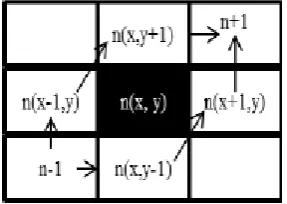
Rather than adding all the adjacent neighbors from current node to open list,
JPS will selectively pick the neighbors based on two lengths. Considering the figure
7(a), current node which is being is expanded is ‘x’, its neighbors(x) = 1,2,3,6,7,8,9
and the parent of ‘x’ is p(x) = 4. We select the neighbors based two lengths. First the
length from parent node p(x) to a neighbor node ‘n’ going via ‘x’ and the second
length from parent node p(x) to neighbor node ‘n’ not going through ‘x’. From the
figure 7(a), the node 5 is not pruned because the length from p(x) to 5 via x is (len (4,
x, 5) = 2) less than length from 4 to 6 not going through 5 (len (4, ! x, 5) = 2.8).
Figure 7(b) shows the example of diagonal pruning rule.
The condition to not select a neighbor for straight move and diagonal move is
give below:
Straight move -> len (p(x), !x, n) <= len (p(x), x, n)
Diagonal move -> len (p(x), !x, n) < len (p(x), x, n)
Figure 7(a): Straight pruning rule Figure 7(b): Diagonal pruning rule
Once we identify the neighbors we apply two pruning rules recursively to all the
18
Straight pruning rule for Forced neighbor:
When there is a straight neighbor of current node ‘x’, we continuous move in that
direction until we encounter the goal node, an obstacle or a forced neighbor for the
expanded node.
Consider the figures 8, if node ‘y’ is the goal node we stop the search, if ‘y’ is an
obstacle we pass a null value which says that the route from the neighbor useless and
when there is a forced neighbor ‘z’ we stop the pruning and pass back ‘y’ as jump
point to ‘x’. The forced neighbor is identified based on two conditions; first it should
not be a natural neighbor of ‘y’ and second the length from ‘x’ to ‘z’ via ‘y’ must be
less then length of ‘x’ to ‘z’ not going via ‘y’ i.e. len(x, y, z) < len(x, !y, z)
Figure 8: Forced neighbor for straight move
Diagonal pruning rule:
When there is a diagonal neighbor of current node ‘x’, we continuous move in
diagonal direction until we encounter the goal node, an obstacle or a forced neighbor
for the expanded node. Figure 9 shows an example of Forced neighbor for diagonal
19
Figure 9: Forced Neighbor for diagonal move
Once we have the jump point nodes for current node ‘x’ we add them to open
list and select the node which as least f(n) value and repeat the process of pruning
until we get the goal node.
JPS is proved to extremely fast in terms solution time compared to A* as it
expands fewer nodes and results show that JPS is 10 times faster than A* algorithm.
The JPS is also proved to be optimal as it produces the shortest path for a unit and it
requires very less memory.
2.2 Multiagent Pathfinding Algorithms:
Multiagent Pathfinding problem (MAPF) deals with finding the routes to all
the units from their respective start node to their respective goal node while avoiding
collision between the units and obstacles on a map. Over the years there have been
many algorithms addressing MAPF problem using two standard approaches.
Centralized approach consists of a centralized controller monitoring all the units to
reach their respective goal nodes while avoiding collision. Decentralized approach
sub divides the problem into single agent runs to reach goal node while avoiding
collision by communicating between the units.
2.2.1 Decentralized Approach:
One of the earliest decentralized approaches was introduced by Stout [12],
20
current neighbor unit. Once all the route for units is generate, the unit tracks back
route to check for collision. If there exists a collision with other unit, the current unit
just reroutes the unit from the node previous to collision node by running A*
algorithm. The same process is repeated for all the units Since A* algorithm is run for
every collision there is massive impact on CPU usage.
To avoid the problem of running A* for every collision Silver [13] introduced
a new algorithm called “Cooperative A*”. A* algorithm is ran on individual units on
a three dimensional space-time, and considering the routes of other units. The
individual routes of units are stored in a data structure “reservation table” which
contains both node on the path and time on which it is being occupied. So while
searching the route for other units, the nodes on the reservation table will become
untraversable at that particular time. When there is a collision between the units, the
unit currently being searched uses a “wait” move. Until the node required by the unit
will not be available, the unit waits at the previous node before collision. Consider the
figure 10(a), with two units ‘A’ and ‘B’ on square grid map with 4 way travel. The
start node and goal node of ‘A’ is S1(0, 0) and G1(3, 3) respectively. And for unit ‘B’,
the start node is S2(0, 1) and goal node is G2(3, 1). When cooperative A* is used on
above map, A* algorithm is ran on unit ‘A’ to generate the path, the same path is
stored in a reservation table along with its time. While running A* on unit ‘B’ all the
expanded nodes from its start node till it reaches the goal node is cross checked
against the reservation table. Since there is no collision the two reach their in optimal
time and path. Consider a similar example as above in figure 10(b), where unit ‘A’ as
same start and goal node, but unit ‘B’ as start node S2(0, 2) and goal node G2(2, 0).
Initially the path for unit ‘A’ is stored in reservation table along with its time, while
21
‘A’ , so the unit ‘B’ waits at node before collision at (0,1) and moves to node (1,1)
when it becomes available.
Figure 10(a): Cooperative A* without collision
Figure 10(b): Cooperative A* with collision
Cooperative A* has some drawbacks in terms of termination of units i.e. the
units would become inactive after reaching the goal and block other units, there is no
prioritization, on when each unit is ran which may impact the units which has longer
path and efficiency of algorithm as the entire path of unit is calculated on a three
22
The above problem in cooperative A* were addressed by Silver [13] with a
“Windowed Hierarchical Cooperative A*”. Here a window of predefined depth is
used while finding the path for individual units i.e. unit’s search is partially stopped
when the window limit is reached, thus allowing the units to be prioritized based on
duration of usage of A* algorithm. By partitioning the search for a unit efficiency of
entire algorithm is increased in terms of time. And finally by using the window, the
units which reach their goal node are still active as long as the window limit is
reached.
Jansen et al. [14] introduce an implicit cooperative pathfinding using direction
maps (DM) which are built on a map. An abstract map is used to run all the units
individually to capture the path and direction of travel which is later used in DM.
Direction maps are data structure with collection of all the direction vectors (DV).
Direction vectors are vectors which give direction to each unit within each traversal of
node, its value ranges from zero to one. The author’s also use movement vectors
(MV) to capture the individual movement between the nodes on the map which could
be any of the 8 directions. Planning of DM is done just the opposite to A* algorithm
where f-cost is used to expand the nodes, while in DM the cost to travel to adjacent
node is changed on both nodes. The main objective of DM is used to find the path
with lower cost when compared shorter path. Thus while traversing on a DM the units
with same direction are grouped together to move to their respective goal nodes The
author’s propose the following formulation using the dot product of DV and MV
which ranges from -1 to 1 for movement from node ‘a’ to node ‘b’
Wab + 0.25 ∙ Wmax (2 - DV a ∙ MV ab - DV b ∙ MV ab)
And `Wmax' is the penalty for units which move in opposite direction to DV ,
23
vector for moving from node `a' to `b', `DV a' is direction vector associated with node
`a' and `DV b' is direction vector associated with edge `b'. Once the DM is built a
single unit, the next unit can use the previous DM to travel on the map. The author’s
state that the dynamic direction maps can be used for learning process has the
direction map will be constantly updated with movements of all units.
One of the most recent works addressing the MAPF problem is proposed by
Bnaya et al. [16], where they introduce a upgrade to Silver [13] “Windowed
Hierarchical Cooperative A*”(WHCA*) called “Conflict oriented Windowed
Hierarchical Cooperative A*” (CO-WHCA*). WHCA* does not consider conflicts
between units in some cases where the window is used for each unit and space-time
node is reserved for the entire path in the reservation table till the window limit. The
space-time node reserved in reservation table may not have any conflicts with the
other units. Secondly in case where the conflict may occur at Window + 1 node for
unit, by then the unit may be physical impossible to avoid the collision. CO-WHCA*
address the above drawbacks by placing the window only when the conflict occurs.
Window is placed only during the conflicts as in case of WHCA* a predefined length
of window size is utilized. One of the conflicting units is selected as a conflict owner
and that unit is allowed to use the window and reserve space-time node in reservation.
Following the initial cycle, after the first reservation table is not erased as in case of
WHCA* and the previous reservation table is utilized while finding routes for next
units. Thus by managing the window only during the conflicts the CO-WHCA*
produces better solution in terms of success-rate, solution cost and time compared to
WHCA*.
The latest algorithm for solution MAPF problem is introduced by
24
map have same direction of travel i.e. on a square grid map of 5x5; all the units have
start nodes on left-hand side and their goal nodes on right-hand side. The main focus
of the RWT algorithm is used to reduce the waiting time of units in a narrow passage
where only few units can pass and rest of units as to wait for their turn to pass. To
reduce the overall time of all units, RWT propose to divide the group of units when
there is a shared passage (i.e. two ways to reach the destination). So the some group
of units take an alternate route then the optimal route to reach their destination. By
doing so the overall solution time is decreased but takes non optimal route to
destination. Consider the figure 11, where there is shared passage ‘A’ and ‘B’, if there
are 20 units entering the large corridor, the RWT algorithm will send 10 units through
passage ‘A’ and rest of units through passage ‘B’ thus reducing overall solution time.
Figure 11: Passage with path ‘A’ and ‘B’[17]
2.2.2 Centralized Approach:
Most of the algorithms using the centralized approach produce an optimal
solution to MAPF problem but fail as the number of units increase on the map. One of
predominate algorithm was introduced by Standley et al. [10], where they introduce
an “operator decomposition” (OD) technique to reduce the branching factor of a
standard A* algorithm which is ran on multi agent environment. By reducing the
25
nodes which would selected during a standard A* run. Even though OD greatly
reduces the number of explored node space, the algorithm will be still exponential. To
tackle this, they introduce independence detection (ID) which utilizes the idea of
decentralized algorithm, by running the units independent to other units. After this
process, they group the units with conflicts and units without. Thus concentrating only
on the conflicting units algorithm reduces overall the solution time. There algorithm
produces an admissible, optimal and complete solution to MAPF problem. Standley et
al. [20] further improved the solution quality by introducing a Maximum Group Size
(MGS) algorithm, which is used to set a maximum size for groups which are created
during ID process, thus allowing conflicting groups to not combine by find a
alterative path. Neither OD+ID nor MGS algorithms could produces optimal solution
for a MAPF, so they introduced an Optimal Anytime algorithm by using MSG
algorithm, where in after finding the solution, the algorithm continues to run until it
finds an optimal solution or until the algorithm terminates. They compared their
algorithm against Hierarchical Cooperative A* (HCA*) to see their algorithm
outperform HCA* in terms of solution quality.
Sharon et al [11] introduce the pruning technique to their previous work called
“Increasing Cost tree Search” (ICTS), where they used increasing cost tree (ICT). By
partitioning the ICT into High level tree which stores all the independent paths of
units and low level tree where they compare the unit’s path with high level tree to
avoid collision and to find optimal solution. There were 4 pruning technique which
was used to improve the solution quality of ICTS algorithm. First was the “Simple
Pairwise Pruning” (SPP), considering a pair of agents ai and aj in the list of agents
from the multi agent problem. Once selected ignoring the rest of the agents the route
26
Ci and Cj. So if there is no immediate solution to the above problem of two agent
search space of MDDij, then the corresponding ICT(n) node can be considered is not
a goal. Second “Enhanced Pairwise Pruning” (EPP), by modifying the SPP, the
pairwise pruning can be improved to perform in worst case also. By modifying the
searching strategy of SPP from depth first search to breadth first search and also by
modifying the single agent MDD's, the EPP removes the invalid nodes from all the
individual MDD. So the k-agent search (higher level search) is improved. Third
“Repeated Enhanced Pairwise Pruning” (REPP), the EPP is continuously iterated to
check until there is no solution for a pair of agent's ai and aj or until there is no single
agent MDD to further iterate in the ICT. Fourth “m-agent Pruning”, where a group of
agents ranging from 2 < m < k can be pruning using the m-agent pruning which
search the m-agent MDD search space using depth first search strategy. So if there is
no solution for the above m-agent pruning. By implementing the pruning techniques
the normal ICST was completed out performed by the ICST with pruning technique.
One most recent works on MAPF problem using centralized approach was
done by Mors et al. [21], where they improved the “push and swap” (P&S) [22]
algorithm. The “push” process is used to move the units towards their respective goals
and “swap” process allows swapping the units without altering the configuration of
units. P&S as some shortcoming on some of instance, during the “swap” process, the
2 swapping units must a node with degree greater than 3 to make perfect swap,
otherwise the one of unit gets stuck or in other instance as to longer route to its
destination. To address the above problems and to produce a complete and optimal
solution, they introduced a “push and rotate” algorithm where in the algorithm is
divided into three phases. In first phase all the disjoint parts are found in the graph
27
on whether a unit from one location can be moved to another location in the graph. In
the second phase, each unit is assigned a sub problem depending on the number of
empty vertices surrounding the sub problem and on whether the units can be moved
out of the sub problem easily. Finally the third phase is to prioritize the units placed in
different sub problems so that the solution can be easily found for the units while
present in bottle neck. Thus solving the entire instances which were not addressed by
P&S and producing a complete algorithm.
2.3 Summary
In this chapter, we have examined some of the relevant papers to our work.
We introduced both the single agent pathfinding and multiagent pathfinding
algorithms. We also examined the two approaches which are employed by various
researchers to address the MAPF problem called centralized approach and
decentralized approach. In the next chapter we are going to explain in detail the most
relevant algorithm Spatially distributed Multiagent Path planning [18] algorithm
which is used to address MAPF problem while managing the transversal of units
28
CHAPTER-3: SPATIALLY DISTRIBUTED MULTIAGENT PATH PLANNING
To address the issue of traversing of units through the narrow corridors in MAPF
problem, Wilt et al [18] introduced a “Spatially Distributed Multiagent Path
Planning” algorithm. The given map is partitioned into Low Contention Area (LCA)
such as open fields in video games, rooms for cleaning robots etc and High
Contention Area (HCA) such as narrow hallway for warehouse robots, bridges in
video games etc. Each of the areas consist of controllers that are responsible for their
respective areas and have knowledge of their area in terms of number of units,
obstacles etc. There is a 1-to-1 mapping between the controllers and areas on the map.
3.1 Spatial Distribution of Map:
Spatial distribution is dividing the map graph G (V, E) with controllers C1 to
Ck where each controller consists of subset of V. The edges connecting within a
controller are called as internal edges and edges connecting between the controllers
are referred to as transition edges. Each controller has the knowledge of its respective
area which is the topology of area and configuration of units within it. There are two
movements of units within a controller that are internal moves and transition moves.
Internal moves are classified into 3 types: first to transfer the unit to its goal with
target macro, second to transfer a unit from current controller to next controller and
third to accept the unit from other controllers. Transition moves are the single step
movement of units through transition edge from one controller to next. The figure 12
shows the two controller1 and controller2. The double ended arrow between the
controllers represents the transition move of unit showing units can travel in both
directions. One of the cases of internal move which is to transfer a unit to its goal ‘G’
29
Figure 12: Spatial distribution of map into controllers and transition move between controllers and internal move
Since each controller has the configuration knowledge of units with it, there is
a need for each controller to know all the units which are arriving and departing from
it. A heuristic guidance is generated by running an individual search for all unit using
A*. This high level path would help the controller to transfer the unit to appropriate
controller and to accept a unit from an appropriate controller. There could be cases
where the units start and goal nodes are within a single controller then the high level
path would consists single controller. In figure 13 we show the high level paths for
two units U1 and U2 with S1, G1 and S2, G2 as start node and goal node respectively.
There are three controllers with name controller 1(C1), controller 2 (C2) and
controller 3(C3). U1 with high level path C1->C2->C3 and U2 with C3 as both its
start and goal nodes are within C3.
30
3.2 High Contention Area:
All the narrow corridors, bridges, narrow hallways on a given map will be
HCA’s. Central core area and buffering area which allows units to wait together
forms a HCA. For a unit to travel through the HCA first it has to arrive at one of the
nodes in buffering area then it is moved to central core area and through the opposite
buffering area. To avoid collision between the units within the HCA, it is divided into
inbound and outbound areas. Based on the direction of travel a unit can take either the
inbound or outbound area.
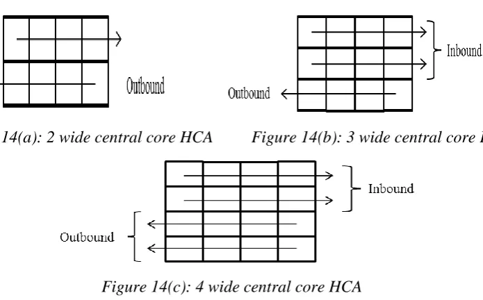
The central core area of HCA is identified on a given map. A pattern of 2, 3
and 4 nodes wide and 8 nodes long both vertical and horizontal is moved over the
map to find all the central core areas for each of the HCA. All three horizontal
patterns with 4 nodes long showing both inbound and outbound direction are shown
in figure 14(a), 14(b) and 14(c).
Figure 14(a): 2 wide central core HCA Figure 14(b): 3 wide central core HCA
Figure 14(c): 4 wide central core HCA
Once the central core area for each HCA is identified, the buffering area must
be created around the central core area for each HCA. The size of 13 nodes is used for
buffering area. Since all units cannot travel through central core there must be a
31
their turn to move. The first step in this process is to divide the central core area of
HCA, for hortizonal cental core the left to right will be inbound and opposite will be
outbound. Following this the first N=13 cells on same side of the direction being
considered will be selected starting from central core area of HCA using Breadth first
search (BFS). Now the HCA is created on the map. Figure 15 shows a HCA with 2
size wide and 4 long vertical central core area represented with ‘C’ cells. Using BFS
on both inbound and outbound direction the buffering area is created around the
central core area which are represeneted with grey cells.
Figure 15: High Contention Area [18]
Each cell in the HCA is given a BFS depth value starting from the first
buffering cell for each direction through the central core area and to other side of
central core area of HCA. In the figure 15, for inbound direction i.e. from down to up
the BFS value for first buffering cell will be 0 and for outbound direction i.e. from up
to down the lowest BFS depth will be at the top buffereing cell. By using BFS depth
of cells in HCA, the units are traversed through the HCA. There are some simple rules
to avoid deadlock and unit starvation such as the prority is always given to unit with
longer time in the controller by moving other units to a empty cell with lower BFS
32
the direction is different value. Units that are on its way out of HCA can either be
transferred to adjacent cell of next controller (only if the cell is avilable) or taken to
end of HCA and then transfer to next controller depending on availability.
3.3 Low Contention Area:
Once the HCA’s are found on map, the rest of area’s can be considered as
LCA’s. The main responsibility of controller of LCA is to transfer the unit to next
HCA controller or to send the unit to its local goal node. Since LCA’s are open area’s
with few obstcales, a modified Cooperative A* [13] is ran for all the units. As the map
is spatially distributed, the standard Cooperative A* [13] cannot be used because of
the following problems. In standard Cooperative A* [13] there is a preset goal node
for each unit and the unit can arrive at its goal at any time, but in spatially distributed
map, the arrival time of unit to its destination cannot be gurantee. So they have
considered the destination of a unit as a disjuctive destinations that are locations
adjacent to existing controller to its next controller. So there could be series of nodes
along each of controller before reaching its actual destination. The other part to
consider is the time, as the availability of nodes to transfer a unit would not be
available at a particular time on a controller. So the disjuctive destination to be
considered as goal state of unit the controller must accept the unit at a arrival time.
Once the units reach their respective goal node, in standard Cooperative A* [13] they
become inactive i.e. they just sit at their goal nodes. Thus making the node not
available to units on its optimal path. In modified Cooperative A* even after reaching
the goal node the unit will be active by replanning a route to goal node, thus allowing
33
3.4 Spatially Distributed Algorithm:
Spatially distributed framework is used to partition the given into High
Contention Area (HCA) and Low Contention Area (LCA). Each area shows a 1-to-1
mapping between the controllers. As stated in the earlier discussiones each controller
communicate with other controller to negotiate the transfer of unit. So there are two
macros to handle the communication in both HCA and LCA controllers with respect
to unit to be transferred, node where unit is accepted and time of arrival of unit. The
pseudo code for both LCA and HCA for accepting a unit is given below. The HCA
accepts the units at particular node and time only if it can keep the previous promise
made to other units. If two units request the same node at same time, then the priority
is given to the unit which asked first and other unit as time wait the transition node for
its turn. As LCA controller’s main responsibilities is to accept unit from HCA and
transfer either to local goal node or to next HCA controller, in pseudocode just
modified Cooperative A* is ran for the particular unit. The location parameter can
either represent a local goal node or the disjunctive destination for next HCA
controller.
34
Algorithm 2: High Contention Area Accepting Unit [18]
3.5 Summary:
In this chapter we have examined the working of “Spatially Distributed
Multiagent Path Planning” (SDP) which address the problem of traversing the units
through the narrow corridor called High Contention Area’s in a MAPF problem. To
do the search for units in Low Contention Area’s (LCA) the authors have proposed a
modified Cooperative A* which is one of earliest algorithm to solve MAPF problem.
In next chapter we propose a novel algorithm called Cooperative Jump Point Search
(Cooperative JPS) which is ran on LCA to find path for units. We see the impact of
Cooperative JPS on the entire SDP framework and modification made to both
![Figure 15: High Contention Area [18]](https://thumb-us.123doks.com/thumbv2/123dok_us/1389309.1171635/48.595.216.405.303.472/figure-high-contention-area.webp)